Workspaces are an efficient model for memory paging in DL4J.
What are workspaces?
ND4J offers an additional memory-management model: workspaces. That allows you to reuse memory for cyclic workloads without the JVM Garbage Collector for off-heap memory tracking. In other words, at the end of the workspace loop, all INDArrays' memory content is invalidated. Workspaces are integrated into DL4J for training and inference.
The basic idea is simple: You can do what you need within a workspace (or spaces), and if you want to get an INDArray out of it (i.e. to move result out of the workspace), you just call INDArray.detach() and you'll get an independent INDArray copy.
Neural Networks
For DL4J users, workspaces provide better performance out of the box, and are enabled by default from 1.0.0-alpha onwards. Thus for most users, no explicit worspaces configuration is required.
To benefit from worspaces, they need to be enabled. You can configure the workspace mode using:
.trainingWorkspaceMode(WorkspaceMode.SEPARATE) and/or .inferenceWorkspaceMode(WorkspaceMode.SINGLE) in your neural network configuration.
The difference between SEPARATE and SINGLE workspaces is a tradeoff between the performance & memory footprint:
SEPARATE is slightly slower, but uses less memory.
SINGLE is slightly faster, but uses more memory.
That said, it’s fine to use different modes for training & inference (i.e. use SEPARATE for training, and use SINGLE for inference, since inference only involves a feed-forward loop without backpropagation or updaters involved).
With workspaces enabled, all memory used during training will be reusable and tracked without the JVM GC interference. The only exclusion is the output() method that uses workspaces (if enabled) internally for the feed-forward loop. Subsequently, it detaches the resulting INDArray from the workspaces, thus providing you with independent INDArray which will be handled by the JVM GC.
Please note: After the 1.0.0-alpha release, workspaces in DL4J were refactored - SEPARATE/SINGLE modes have been deprecated, and users should use ENABLED instead.
Garbage Collector
If your training process uses workspaces, we recommend that you disable (or reduce the frequency of) periodic GC calls. That can be done like so:
Put that somewhere before your model.fit(...) call.
ParallelWrapper & ParallelInference
For ParallelWrapper, the workspace-mode configuration option was also added. As such, each of the trainer threads will use a separate workspace attached to the designated device.
Iterators
We provide asynchronous prefetch iterators, AsyncDataSetIterator and AsyncMultiDataSetIterator, which are usually used internally.
These iterators optionally use a special, cyclic workspace mode to obtain a smaller memory footprint. The size of the workspace, in this case, will be determined by the memory requirements of the first DataSet coming out of the underlying iterator, whereas the buffer size is defined by the user. The workspace will be adjusted if memory requirements change over time (e.g. if you’re using variable-length time series).
Caution: If you’re using a custom iterator or the RecordReader, please make sure you’re not initializing something huge within the first next() call. Do that in your constructor to avoid undesired workspace growth.
Caution: With AsyncDataSetIterator being used, DataSets are supposed to be used before calling the next() DataSet. You are not supposed to store them, in any way, without the detach() call. Otherwise, the memory used for INDArrays within DataSet will be overwritten within AsyncDataSetIterator eventually.
If for some reason you don’t want your iterator to be wrapped into an asynchronous prefetch (e.g. for debugging purposes), special wrappers are provided: AsyncShieldDataSetIterator and AsyncShieldMultiDataSetIterator. Basically, those are just thin wrappers that prevent prefetch.
Evaluation
Usually, evaluation assumes use of the model.output() method, which essentially returns an INDArray detached from the workspace. In the case of regular evaluations during training, it might be better to use the built-in methods for evaluation. For example:
This piece of code will run a single cycle over iteratorTest, and it will update both (or less/more if required by your needs) IEvaluation implementations without any additional INDArray allocation.
Workspace Destruction
There are also some situations, say, where you're short on RAM, and might want do release all workspaces created out of your control; e.g. during evaluation or training.
That could be done like so: Nd4j.getWorkspaceManager().destroyAllWorkspacesForCurrentThread();
This method will destroy all workspaces that were created within the calling thread. If you've created workspaces in some external threads on your own, you can use the same method in that thread, after the workspaces are no longer needed.
Workspace Exceptions
If workspaces are used incorrectly (such as a bug in a custom layer or data pipeline, for example), you may see an error message such as:
DL4J's LayerWorkspaceMgr
DL4J's Layer API includes the concept of a "layer workspace manager".
The idea with this class is that it allows us to easily and precisely control the location of a given array, given different possible configurations for the workspaces. For example, the activations out of a layer may be placed in one workspace during inference, and another during training; this is for performance reasons. However, with the LayerWorkspaceMgr design, implementers of layers don't need to worry about this.
What does this mean in practice? Usually it's quite simple...
When returning activations (activate(boolean training, LayerWorkspaceMgr workspaceMgr) method), make sure the returned array is defined in ArrayType.ACTIVATIONS (i.e., use LayerWorkspaceMgr.create(ArrayType.ACTIVATIONS, ...) or similar)
When returning activation gradients (backpropGradient(INDArray epsilon, LayerWorkspaceMgr workspaceMgr)), similarly return an array defined in ArrayType.ACTIVATION_GRAD
You can also leverage an array defined in any workspace to the appropriate workspace using, for example, LayerWorkspaceMgr.leverageTo(ArrayType.ACTIVATIONS, myArray)
Note that if you are not implementing a custom layer (and instead just want to perform forward pass for a layer outside of a MultiLayerNetwork/ComputationGraph) you can use LayerWorkspaceMgr.noWorkspaces().
// this will limit frequency of gc calls to 5000 milliseconds
Nd4j.getMemoryManager().setAutoGcWindow(5000)
// OR you could totally disable it
Nd4j.getMemoryManager().togglePeriodicGc(false);
ParallelWrapper wrapper = new ParallelWrapper.Builder(model)
// DataSets prefetching options. Buffer size per worker.
.prefetchBuffer(8)
// set number of workers equal to number of GPUs.
.workers(2)
// rare averaging improves performance but might reduce model accuracy
.averagingFrequency(5)
// if set to TRUE, on every averaging model score will be reported
.reportScoreAfterAveraging(false)
// 3 options here: NONE, SINGLE, SEPARATE
.workspaceMode(WorkspaceMode.SINGLE)
.build();
Evaluation eval = new Evaluation(outputNum);
ROC roceval = new ROC(outputNum);
model.doEvaluation(iteratorTest, eval, roceval);
org.nd4j.linalg.exception.ND4JIllegalStateException: Op [set] Y argument uses leaked workspace pointer from workspace [LOOP_EXTERNAL]
For more details, see the ND4J User Guide: nd4j.org/userguide#workspaces-panic
Elementwise Operations
Elementwise operations are more intuitive than vectorwise operations, because the elements of one matrix map clearly onto the other, and to obtain the result, you have to perform just one arithmetical operation.
With vectorwise matrix operations, you will have to first build intuition and also perform multiple steps. There are two basic types of matrix multiplication: inner (dot) product and outer product. The inner product results in a matrix of reduced dimensions, the outer product results in one of expanded dimensions. A helpful mnemonic: Expand outward, contract inward.
Inner product
Unlike Hadamard products, which require that both matrices have equal rows and columns, inner products simply require that the number of columns of the first matrix equal the number of rows of the second. For example, this works
Notice a 1 x 2 row times a 2 x 1 column produces a scalar. This operation reduces the dimensions to 1,1. You can imagine rotating the row vector [1.0 ,2.0] clockwise to stand on its end, placed against the column vector. The two top elements are then multiplied by each other, as are the bottom two, and the two products are added to consolidate in a single scalar.
In ND4J, you would create the two vectors like this:
And multiply them like this
Notice ND4J code mirrors the equation in that nd * nd2 is row vector times column vector. The method is mmul, rather than the mul we used for elementwise operations, and the extra “m” stands for “matrix.”
Now let’s take the same operation, while adding an additional column to a new array we’ll call nd4.
Now let’s add an extra row to the first matrix, call it nd3, and multiply it by nd4
The equation will look like this
Taking the outer product of the two vectors we first worked with is as simple as reversing their order.
It turns out the multiplying nd2 by nd is the same as multiplying it by two nd’s stacked on top of each other. That’s an outer product. As you can see, outer products also require fewer operations, since they don’t combine two products into one element in the final matrix.
A few aspects of ND4J code should be noted here. Firstly, the method mmul takes two parameters.
which could be expressed like this
which is the same as this line
Using the second parameter to specify the nd-array to which the product should be assigned is a convention common in ND4J.
Tensors
A vector, that column of numbers we feed into neural nets, is simply a subclass of a more general mathematical structure called a tensor. A tensor is a multidimensional array.
You are already familiar with a matrix composed of rows and columns: the rows extend along the y axis and the columns along the x axis. Each axis is a dimension. Tensors have additional dimensions.
Tensors also have a so-called rank: a scalar, or single number, is of rank 0; a vector is rank 1; a matrix is rank 2; and entities of rank 3 and above are all simply called tensors.
It may be helpful to think of a scalar as a point, a vector as a line, a matrix as a plane, and tensors as objects of three dimensions or more. A matrix has rows and columns, two dimensions, and therefore is of rank 2. A three-dimensional tensor, such as those we use to represent color images, has channels, rows and columns, and therefore counts as rank 3.
As mathematical objects with multiple dimensions, tensors have a shape, and we specify that shape by treating tensors as n-dimensional arrays.
With ND4J, we do that by creating a new nd array and feeding it data, shape and order as its parameters. In pseudo code, this would be
In real code, this line
creates an array with four elements, whose shape is 2 by 2, and whose order is “row major”, or rows first, which is the default in C. (In contrast, Fortran uses “column major” ordering, and could be specified with an ‘f’ as the third parameter.) The distinction between thetwo orderings, for the array created above, is best illustrated with a table:
Once we create an n-dimensional array, we may want to work with slices of it. Rather than copying the data, which is expensive, we can simply “view” muli-dimensional slices. A slice of array “a” could be defined like this:
which would give you the first 5 channels, rows 3 to 4 and columns 6 to 7, and so forth for n dimensions, which each individual dimension’s slice starting before the colon and ending after it.
Now, while it is useful to imagine matrices as two-dimensional planes, and 3-D tensors are cubic volumes, we store all tensors as a linear buffer. That is, they are all flattened to a row of numbers.
For that linear buffer, we specify something called stride. Stride tells the computation layer how to interpret the flattened representation. It is the number of elements you skip in the buffer to get to the next channel or row or column. There’s a stride for each dimension.
Here’s a brief video summarizing how tensors are converted into linear byte buffers for ND4J.
The word tensor derives from the Latin tendere, or “to stretch”; therefore, tensor relates to that which stretches, the stretcher. Tensor was introduced to English from the German in 1915, after being coined by Woldemar Voigt in 1898. The mathematical object is called a tensor because an early application of the idea was the study of materials stretching under tension.
Tutorials
Deeplearning4j Tutorials
While Deeplearning4j is written in Java, the Java Virtual Machine (JVM) lets you import and share code in other JVM languages. These tutorials are written in Scala, the de facto standard for data science in the Java environment. There’s nothing stopping you from using any other interpreter such as Java, Kotlin, or Clojure.
If you’re coming from non-JVM languages like Python or R, you may want to read about how the JVM works before using these tutorials. Knowing the basic terms such as classpath, virtual machine, “strongly-typed” languages, and functional programming will help you debug, as well as expand on the knowledge you gain here. If you don’t know Scala and want to learn it, Coursera has a great course named .
Eclipse DeepLearning4J
Eclipse Deeplearning4j is the first commercial-grade, open-source, distributed deep-learning library written for Java and Scala. Integrated with Hadoop and Apache Spark, DL4J brings AI to business environments for use on distributed GPUs and CPUs.
Distributed
DL4J takes advantage of the latest distributed computing frameworks including Apache Spark and Hadoop to accelerate training. On multi-GPUs, it is equal to Caffe in performance.
Open Source
The libraries are completely open-source, Apache 2.0, and maintained by the developer community and Konduit team.
JVM/Python/C++
The tutorials are currently being reworked. You will likely find stumbling points. If you need any support while working through them, feel free to ask questions on https://community.konduit.ai/.
Deeplearning4j is written in Java and is compatible with any JVM language, such as Scala, Clojure or Kotlin. The underlying computations are written in C, C++ and Cuda. Keras will serve as the Python API.
Deep neural nets are capable of record-breaking accuracy. For a quick neural net introduction, please visit our overview page. In a nutshell, Deeplearning4j lets you compose deep neural nets from various shallow nets, each of which form a so-called `layer`. This flexibility lets you combine variational autoencoders, sequence-to-sequence autoencoders, convolutional nets or recurrent nets as needed in a distributed, production-grade framework that works with Spark and Hadoop on top of distributed CPUs or GPUs.
There are a lot of parameters to adjust when you're training a deep-learning network. We've done our best to explain them, so that Deeplearning4j can serve as a DIY tool for Java, Scala, Clojure and Kotlin programmers.
Tensors are generalizations of scalars (that have no indices), vectors (that have exactly one index), and matrices (that have exactly two indices) to an arbitrary number of indices. - Mathworld
tensor, n. a mathematical object analogous to but more general than a vector, represented by an array of components that are functions of the coordinates of a space.
Hardware setup for Eclipse Deeplearning4j, including GPUs and CUDA.
ND4J backends for GPUs and CPUs
You can choose GPUs or native CPUs for your backend linear algebra operations by changing the dependencies in ND4J's POM.xml file. Your selection will affect both ND4J and DL4J being used in your application.
If you have CUDA v9.2+ installed and NVIDIA-compatible hardware, then your dependency declaration will look like:
As of now, the artifactId for the CUDA versions can be one of nd4j-cuda-9.2, nd4j-cuda-10.0, nd4j-cuda-10.1 or nd4j-cuda-10.2.
You can also find the available CUDA versions via Maven Central search or in the .
Otherwise you will need to use the native implementation of ND4J as a CPU backend:
If you are developing your project on multiple operating systems/system architectures, you can add -platform to the end of your artifactId which will download binaries for most major systems.
See our page on .
Check the NVIDIA guides for instructions on setting up CUDA on the NVIDIA .
CPU and AVX
CPU and AVX support in ND4J/Deeplearning4j
AVX (Advanced Vector Extensions) is a set of CPU instructions for accelerating numerical computations. See for more details.
Note that AVX only applies to nd4j-native (CPU) backend for x86 devices, not GPUs and not ARM/PPC devices.
Why AVX matters: performance. You want to use the version of ND4J compiled with the highest level of AVX supported by your system.
AVX support for different CPUs - summary:
Most modern x86 CPUs: AVX2 is supported
About
Facts and introduction to Eclipse Deeplearning4j, the top JVM deep learning framework.
Eclipse Deeplearning4j is an open-source, distributed deep-learning project in Java and Scala spearheaded by the people at , a business intelligence and enterprise software firm. We're a team of data scientists, deep-learning specialists, Java systems engineers and semi-sentient robots.
There are a lot of knobs to turn when you're training a distributed deep-learning network. We've done our best to explain them, so that Eclipse Deeplearning4j can serve as a DIY tool for Java, Scala and Clojure programmers working on Hadoop and other file systems.
Deeplearning4j has been featured in , , , , , and .
If you plan to publish an academic paper and wish to cite Deeplearning4j, please use this format:
Eclipse Deeplearning4j Development Team. Deeplearning4j: Open-source distributed deep learning for the JVM, Apache Software Foundation License 2.0.
Profiling supported by
Multilayer Network
Simple and sequential network configuration.
The MultiLayerNetwork class is the simplest network configuration API available in Eclipse Deeplearning4j. This class is useful for beginners or users who do not need a complex and branched network graph.
You will not want to use MultiLayerNetwork configuration if you are creating complex loss functions, using graph vertices, or doing advanced training such as a triplet network. This includes popular complex networks such as InceptionV4.
The example below shows how to build a simple linear classifier using DenseLayer (a basic multiperceptron layer).
You can also create convolutional configurations:
SBT, Gradle, & Others
Configure the build tools for Deeplearning4j.
While we encourage Deeplearning4j, ND4J and DataVec users to employ Maven, it's worthwhile documenting how to configure build files for other tools, like Ivy, Gradle and SBT -- particularly since Google prefers Gradle over Maven for Android projects.
The instructions below apply to all DL4J and ND4J submodules, such as deeplearning4j-api, deeplearning4j-scaleout, and ND4J backends.
You can use Deeplearning4j with Gradle by adding the following to your build.gradle in the dependencies block:
Add a backend by adding the following:
You can also swap the standard CPU implementation for .
You can use Deeplearning4j with SBT by adding the following to your build.sbt:
Add a backend by adding the following:
Optimizers
Supported Keras optimizers
All standard Keras optimizers are supported, but importing custom TensorFlow optimizers won't work:
MultiLayerConfiguration conf = new NeuralNetConfiguration.Builder()
.seed(seed)
.optimizationAlgo(OptimizationAlgorithm.STOCHASTIC_GRADIENT_DESCENT)
.learningRate(learningRate)
.updater(Updater.NESTEROVS).momentum(0.9)
.list()
.layer(0, new DenseLayer.Builder().nIn(numInputs).nOut(numHiddenNodes)
.weightInit(WeightInit.XAVIER)
.activation("relu")
.build())
.layer(1, new OutputLayer.Builder(LossFunction.NEGATIVELOGLIKELIHOOD)
.weightInit(WeightInit.XAVIER)
.activation("softmax").weightInit(WeightInit.XAVIER)
.nIn(numHiddenNodes).nOut(numOutputs).build())
.pretrain(false).backprop(true).build();
Usage
Some high-end server CPUs: AVX512 may be supported
Old CPUs (pre 2012) and low power x86 (Atom, Celeron): No AVX support (usually)
Note that CPUs supporting later versions of AVX include all earlier versions also. This means it's possible run a generic x86 or AVX2 binary on a system supporting AVX512. However it is not possible to run binaries built for later versions (such as avx512) on a CPU that doesn't have support for those instructions.
In version 1.0.0-beta6 and later you may get a warning as follows, if AVX is not configured optimally:
As noted earlier, for best performance you should use the version of ND4J that matches your CPU's supported AVX level.
ND4J defaults configuration (when just including the nd4j-native or nd4j-native-platform dependencies without maven classifier configuration) is "generic x86" (no AVX) for nd4j/nd4j-platform dependencies.
To configure AVX2 and AVX512, you need to specify a classifier for the appropriate architecture.
The following binaries (nd4j-native classifiers) are provided for x86 architectures:
Generic x86 (no AVX): linux-x86_64, windows-x86_64, macosx-x86_64
NOTE: You'll still need to download ND4J, DataVec and Deeplearning4j, or doubleclick on the their respective JAR files file downloaded by Maven / Ivy / Gradle, to install them in your Eclipse installation.
MultiLayerConfiguration.Builder builder = new NeuralNetConfiguration.Builder()
.seed(seed)
.regularization(true).l2(0.0005)
.learningRate(0.01)
.weightInit(WeightInit.XAVIER)
.optimizationAlgo(OptimizationAlgorithm.STOCHASTIC_GRADIENT_DESCENT)
.updater(Updater.NESTEROVS).momentum(0.9)
.list()
.layer(0, new ConvolutionLayer.Builder(5, 5)
//nIn and nOut specify depth. nIn here is the nChannels and nOut is the number of filters to be applied
.nIn(nChannels)
.stride(1, 1)
.nOut(20)
.activation("identity")
.build())
.layer(1, new SubsamplingLayer.Builder(SubsamplingLayer.PoolingType.MAX)
.kernelSize(2,2)
.stride(2,2)
.build())
.layer(2, new ConvolutionLayer.Builder(5, 5)
//Note that nIn need not be specified in later layers
.stride(1, 1)
.nOut(50)
.activation("identity")
.build())
.layer(3, new SubsamplingLayer.Builder(SubsamplingLayer.PoolingType.MAX)
.kernelSize(2,2)
.stride(2,2)
.build())
.layer(4, new DenseLayer.Builder().activation("relu")
.nOut(500).build())
.layer(5, new OutputLayer.Builder(LossFunctions.LossFunction.NEGATIVELOGLIKELIHOOD)
.nOut(outputNum)
.activation("softmax")
.build());
*********************************** CPU Feature Check Warning ***********************************
Warning: Initializing ND4J with Generic x86 binary on a CPU with AVX/AVX2 support
Using ND4J with AVX/AVX2 will improve performance. See deeplearning4j.org/cpu for more details
Or set environment variable ND4J_IGNORE_AVX=true to suppress this warning
************************************************************************************************
With deep learning, we can compose a deep neural network to suit the input data and its features. The goal is to train the network on the data to make predictions, and those predictions are tied to the outcomes that you care about; i.e. is this transaction fraudulent or not, or which object is contained in the photo? There are different techniques to configure a neural network, and all of them build a relational hierarchy between the inputs and outputs.
In this tutorial, we are going to configure the simplest neural network and that is logistic regression model network.
Regression is a process that helps show the relations between the independent variables (inputs) and the dependent variables (outputs). Logistic regression is one in which the dependent variable is categorical rather than continuous - meaning that it can predict only a limited number of classes or categories, like a switch you flip on or off. For example, it can predict that an image contains a cat or a dog, or it can classify input in ten buckets with the integers 0 through 9.
A simple logistic regression calculates x*w + b = y. Where x is an instance of input data, w is the weight or coefficient that transforms that input, b is the bias and y is the output, or prediction about the data. The biological terms show how this artificial neuron loosely maps to a neuron in the human brain. The most important point is how data flows through and is transformed by this structure.
We’re going to configure the simplest network, with just one input layer and one output layer, to show how logistic regression works.
We are going to first build the layers and then feed these layers into the network configuration.
You may be wondering why didn’t we write any code for building our input layer. The input layer is only a set of inputs values fed into the network. It doesn’t perform a calculation. It’s just an input sequence (raw or pre-processed data) coming into the network, data to be trained on or to be evaluated. Later, we are going to work with data iterators, which feed input to a network in a specific pattern, and which can be thought of as an input layer of the network.
Eclipse Contributors
IP/Copyright requirements for Eclipse Foundation Projects
Contributors (anyone who wants to commit code to the repository) need to do two things, before their code can be merged:
Sign the Eclipse Contributor Agreement (once)
Sign commits (each time)
Why Is This Required?
These two requirements must be satisfied for all Eclipse Foundation projects, not just DL4J and ND4J. A full list of Eclipse Foundation Projects can be found here:
By signing the ECA, you are essentially asserting that the code you are submitting is something that either you wrote, or that you have the right to contribute to the project. This is a necessary legal protection to avoid copyright issues.
By signing your commits, you are asserting that the code in that particular commit is your own.
You only need to sign the Eclipse Contributor Agreement (ECA) once. Here's the process:
Step 1: Sign up for an Eclipse account
This can be done at
Note: You must register using the same email as your GitHub account (the GitHub account you want to submit pull requests from).
Step 2: Sign the ECA
Go to and follow the instructions.
There are a few ways to sign commits. Note that you can use any of these aoptions.
Option 1: Use -s When Committing on Command Line
Signing commits here is simple:
Note the use of -s (lower case s) - upper-case S (i.e., -S) is for GPG signing (see below).
Option 2: Set up Bash Alias (or Windows cmd Alias) for Automated Signing
For example, you could set up the following alias in Bash:
Then committing would be done with the following:
For Windows command line, similar options are available through a few mechanisms (see )
One simple way is to create a gcm.bat file with the following contents, and add it to your system path:
You can then commit using the same process as above (i.e., gcm "My Commit")
Option 3: Use GPG Signing
For details on GPG signing, see
Note that this option can be combined with aliases (above), as in alias gcm='git commit -S -m' - note the upper case -S for GPG signing.
Option 4: Commit using IntelliJ with Auto Signing
IntelliJ can be used to perform git commits, including through signed commits. See for details.
After performing a commit, you can check in a few different ways. One way is to use git log --show-signature -1 to show the signature for the last commit (use -5 to show the last 5 commits, for example)
The output will look like:
The top commit is unsigned, and the bottom commit is signed (note the presence of the Signed-off-by).
If you forgot to sign the last commit, you can use the following command:
Suppose your branch has 3 new commits, all of which are unsigned:
One simple way is to squash and sign these commits. To do this for the last 3 commits, use the following: (note you might want to make a backup first)
The result:
You can confirm that the commit is signed using git log -1 --show-signature as shown earlier.
Note that your commits will be squashed once they are merged to master anyway, so the loss of the commit history does not matter.
If you are updating an existing PR, you may need to force push using -f (as in git push X -f).
Snapshots
Using daily builds for access to latest Eclipse Deeplearning4j features.
We provide automated daily builds of repositories such as ND4J, DataVec, DeepLearning4j, RL4J etc. So all the newest functionality and most recent bug fixes are released daily.
Snapshots work like any other Maven dependency. The only difference is that they are served from a custom repository rather than from Maven Central.
Due to ongoing development, snapshots should be considered less stable than releases: breaking changes or bugs can in principle be introduced at any point during the course of normal development. Typically, releases (not snapshots) should be used when possible, unless a bug fix or new feature is required.
Step 1: To use snapshots in your project, you should add snapshot repository information like this to your pom.xml file:
Step 2: Make sure to specify the snapshot version. We follow a simple rule: If the latest stable release version is A.B.C, the snapshot version will be A.B.(C+1)-SNAPSHOT. The current snapshot version is 1.0.0-SNAPSHOT. For more details on the repositories section of the pom.xml file, see
If using properties like the DL4J examples, change: From version:
To version:
Sample pom.xml using Snapshots
A sample pom.xml is provided here: This has been taken from the DL4J standalone sample project and modified using step 1 and 2 above. The original (using the last release) can be found
Both -platform (all operating systems) and single OS (non-platform) snapshot dependencies are released. Due to the multi-platform build nature of snapshots, it is possible (though rare) for the -platform artifacts to temporarily get out of sync, which can cause build issues.
If you are building and deploying on just one platform, it is safter use the non-platform artifacts, such as:
Two commands that might be useful when using snapshot dependencies in Maven is as follows: 1. -U - for example, in mvn package -U. This -U option forces Maven to check (and if necessary, download) of new snapshot releases. This can be useful if you need the be sure you have the absolute latest snapshot release. 2. -nsu - for example, in mvn package -nsu. This -nsu option stops Maven from checking for snapshot releases. Note however your build will only succeed with this option if you have some snapshot dependencies already downloaded into your local Maven cache (.m2 directory)
An alternative approach to (1) is to set <updatePolicy>always</updatePolicy> in the <repositories> section found earlier in this page. An alternative approach to (2) is to set <updatePolicy>never</updatePolicy> in the <repositories> section found earlier in this page.
Snapshots will not work with Gradle. You must use Maven to download the files. After that, you may try using your local Maven repository with mavenLocal().
A bare minimum file like this:
should work in theory, but it does not. This is due to . Gradle with snapshots and Maven classifiers appears to be a problem.
Of note when using the nd4j-native backend on Gradle (and SBT - but not Maven), you need to add openblas as a dependency. We do this for you in the -platform pom. Reference the -platform pom to double check your dependencies. Note that these are version properties. See the <properties> section of the pom for current versions of the openblas and javacpp presets required to run nd4j-native.
Contribute
How to contribute to the Eclipse Deeplearning4j source code.
Prerequisites
Before contributing, make sure you know the structure of all of the Eclipse Deeplearning4j libraries. As of early 2018, all libraries now live in the Deeplearning4j monorepo. These include:
DeepLearning4J: Contains all of the code for learning neural networks, both on a single machine and distributed.
ND4J: “N-Dimensional Arrays for Java”. ND4J is the mathematical backend upon which DL4J is built. All of DL4J’s neural networks are built using the operations (matrix multiplications, vector operations, etc) in ND4J. ND4J is how DL4J supports both CPU and GPU training of networks, without any changes to the networks themselves. Without ND4J, there would be no DL4J.
DataVec: DataVec handles the data import and conversion side of the pipeline. If you want to import images, video, audio or simply CSV data into DL4J: you probably want to use DataVec to do this.
Arbiter: Arbiter is a package for (amongst other things) hyperparameter optimization of neural networks. Hyperparameter optimization refers to the process of automating the selection of network hyperparameters (learning rate, number of layers, etc) in order to obtain good performance.
We also have an extensive examples repository at .
There are numerous ways to contribute to DeepLearning4J (and related projects), depending on your interests and experince. Here’s some ideas:
Add new types of neural network layers (for example: different types of RNNs, locally connected networks, etc)
Add a new training feature
Bug fixes
DL4J examples: Is there an application or network architecture that we don’t have examples for?
There are a number of different ways to find things to work on. These include:
Looking at the issue trackers:
Reviewing our Roadmap
Talking to the developers on the
Before you dive in, there’s a few things you need to know. In particular, the tools we use:
Maven: a dependency management and build tool, used for all of our projects. See this for details on Maven.
Git: the version control system we use
Project Lombok: Project Lombok is a code generation/annotation tool that is aimed to reduce the amount of ‘boilerplate’ code (i.e., standard repeated code) needed in Java. To work with source, you’ll need to install the Project Lombok plugin for your IDE
Things to keep in mind:
Code should be Java 7 compliant
If you are adding a new method or class: add JavaDocs
You are welcome to add an author tag for significant additions of functionality. This can also help future contributors, in case they need to ask questions of the original author. If multiple authors are present for a class: provide details on who did what (“original implementation”, “added feature x” etc)
Custom Layers
Extend DL4J functionality for custom layers.
There are two components to adding a custom layer:
Adding the layer configuration class: extends org.deeplearning4j.nn.conf.layers.Layer
Adding the layer implementation class: implements org.deeplearning4j.nn.api.Layer
The configuration layer ((1) above) class handles the settings. It's the one you would use when constructing a MultiLayerNetwork or ComputationGraph. You can add custom settings here, and use them in your layer.
The implementation layer ((2) above) class has parameters, and handles network forward pass, backpropagation, etc. It is created from the org.deeplearning4j.nn.conf.layers.Layer.instantiate(...) method. In other words: the instantiate method is how we go from the configuration to the implementation; MultiLayerNetwork or ComputationGraph will call this method when initializing the
An example of these are CustomLayer (the configuration class) and CustomLayerImpl (the implementation class). Both of these classes have extensive comments regarding their methods.
You'll note that in Deeplearning4j there are two DenseLayer clases, two GravesLSTM classes, etc: the reason is because one is for the configuration, one is for the implementation. We have not followed this "same name" pattern here to hopefully avoid confusion.
Once you have added a custom layer, it is necessary to run some tests to ensure it is correct.
These tests should at a minimum include the following:
Tests to ensure that the JSON configuration (to/from JSON) works correctly
This is necessary for networks with your custom layer to function with both
model serialization (saving) and Spark training.
Gradient checks to ensure that the implementation is correct.
A full custom layer example is available in our .
Get Started
Getting started with model import.
tf.keras import is not supported yet.
Below is a video tutorial demonstrating working code to load a Keras model into Deeplearning4j and validating the working network. Instructor Tom Hanlon provides an overview of a simple classifier over Iris data built in Keras with a Theano backend, and exported and loaded into Deeplearning4j:
If you have trouble viewing the video, please click here to view it on YouTube.
The mapping of Keras to DL4J activation functions is defined in
Regularizers
Supported Keras regularizers.
All [Keras regularizers] are supported by DL4J model import:
l1
l2
l1_l2
Mapping of regularizers can be found in .
Feed Forward Networks
In our previous tutorial, we learned about a very simple neural network model - the logistic regression model. Although you can solve many tasks with a simple model like that, most of the problems require a much complex network configuration. Typical Deep leaning model consists of many layers between the inputs and outputs. In this tutorial, we are going to learn about one of those configuration i.e. Feed-forward neural networks.
Feed-forward networks are those in which there is not cyclic connection between the network layers. The input flows forward towards the output after going through several intermediate layers. A typical feed-forward network looks like this:
Here you can see a different layer named as a hidden layer. The layers in between our input and output layers are called hidden layers. It’s called hidden because we don’t directly deal with them and hence not visible. There can be more than one hidden layer in the network.
Just as our softmax activation after our output layer in the previous tutorial, there can be activation functions between each layer of the network. They are responsible to allow (activate) or disallow our network output to the next layer node. There are different activation functions such as sigmoid and relu etc.
cuDNN
Using the NVIDIA cuDNN library with DL4J.
Deeplearning4j supports CUDA but can be further accelerated with cuDNN. Most 2D CNN layers (such as ConvolutionLayer, SubsamplingLayer, etc), and also LSTM and BatchNormalization layers support CuDNN.
The only thing we need to do to have DL4J load cuDNN is to add a dependency on deeplearning4j-cuda-9.2, deeplearning4j-cuda-10.0, deeplearning4j-cuda-10.1,or deeplearning4j-cuda-10.2, for example:
or
or
or
Vertices
Computation graph nodes for advanced configuration.
In Eclipse Deeplearning4j a vertex is a type of layer that acts as a node in a ComputationGraph. It can accept multiple inputs, provide multiple outputs, and can help construct popular networks such as InceptionV4.
L2NormalizeVertex performs L2 normalization on a single input.
L2Vertex calculates the L2 least squares error of two inputs.
t-SNE Visualization
Data visualizaiton with t-SNE with higher dimensional data.
(t-SNE) is a data-visualization tool created by Laurens van der Maaten at Delft University of Technology.
While it can be used for any data, t-SNE (pronounced Tee-Snee) is only really meaningful with labeled data, which clarify how the input is clustering. Below, you can see the kind of graphic you can generate in DL4J with t-SNE working on MNIST data.
Look closely and you can see the numerals clustered near their likes, alongside the dots.
Here's how t-SNE appears in Deeplearning4j code.
Here is an image of the tsne-standard-coords.csv file plotted using gnuplot.
Backend
ND4J works atop so-called backends, or linear-algebra libraries, such as Native nd4j-native and nd4j-cuda-$SOME_CUDA_VERSION (usually the 2 most recent cuda versions) (GPUs), which you can select by pasting the .
A Java , which is baked into the language itself, tells Java that the backend exists. It’s not necessary to concern yourself with how ND4J backends load and perform other basic functions, but you can explore .
The core configurations for each backend are specified in a properties file.
A few more points:
Sequential Model
Importing the functional model.
Let's say you start with defining a simple MLP using Keras:
In Keras there are several ways to save a model. You can store the whole model (model definition, weights and training configuration) as HDF5 file, just the model configuration (as JSON or YAML file) or just the weights (as HDF5 file). Here's how you do each:
If you decide to save the full model, you will have access to the training configuration of the model, otherwise you don't. So if you want to further train your model in DL4J after import, keep that in mind and use model.save(...) to persist your model.
Let's start with the recommended way, loading the full model back into DL4J (we assume it's on your class path):
In case you didn't compile your Keras model, it will not come with a training configuration. In that case you need to explicitly tell model import to ignore training configuration by setting the enforceTrainingConfig flag to false like this:
Functional Model
Importing the functional model.
Let's say you start with defining a simple MLP using Keras' functional API:
In Keras there are several ways to save a model. You can store the whole model (model definition, weights and training configuration) as HDF5 file, just the model configuration (as JSON or YAML file) or just the weights (as HDF5 file). Here's how you do each:
If you decide to save the full model, you will have access to the training configuration of the model, otherwise you don't. So if you want to further train your model in DL4J after import, keep that in mind and use model.save(...) to persist your model.
Let's start with the recommended way, loading the full model back into DL4J (we assume it's on your class path):
In case you didn't compile your Keras model, it will not come with a training configuration. In that case you need to explicitly tell model import to ignore training configuration by setting the enforceTrainingConfig flag to false like this:
Testing performance and identifying bottlenecks or areas to improve
Reviewing recent papers and blog posts on training features, network architectures and applications
Reviewing the website and examples - what seems missing, incomplete, or would simply be useful (or cool) to have?
VisualVM: A profiling tool, most useful to identify performance issues and bottlenecks.
IntelliJ IDEA: This is our IDE of choice, though you may of course use alternatives such as Eclipse and NetBeans. You may find it easier to use the same IDE as the developers in case you run into any issues. But this is up to you.
Provide informative comments throughout your code. This helps to keep all code maintainable.
Any new functionality should include unit tests (using JUnit) to test your code. This should include edge cases.
If you add a new layer type, you must include numerical gradient checks, as per these unit tests. These are necessary to confirm that the calculated gradients are correct
If you are adding significant new functionality, consider also updating the relevant section(s) of the website, and providing an example. After all, functionality that nobody knows about (or nobody knows how to use) isn’t that helpful. Adding documentation is definitely encouraged when appropriate, but strictly not required.
If you are unsure about something - ask us on the community forums!
For example, in Triplet Embedding you can input an anchor and a pos/neg class and use two parallel L2 vertices to calculate two real numbers which can be fed into a LossLayer to calculate TripletLoss.
Adds the ability to reshape and flatten the tensor in the computation graph. This is the equivalent to the next layer. ReshapeVertex also ensures the shape is valid for the backward pass.
A ScaleVertex is used to scale the size of activations of a single layer
For example, ResNet activations can be scaled in repeating blocks to keep variance under control.
A ShiftVertex is used to shift the activations of a single layer
One could use it to add a bias or as part of some other calculation. For example, Highway Layers need them in two places. One, it’s often useful to have the gate weights have a large negative bias. (Of course for this, we could just initialize the biases that way.) But, also it needs to do this: (1-sigmoid(weight input + bias)) () input + sigmoid(weight input + bias) () activation(w2 input + bias) (() is hadamard product) So, here, we could have
StackVertex allows for stacking of inputs so that they may be forwarded through a network. This is useful for cases such as Triplet Embedding, where shared parameters are not supported by the network.
This vertex will automatically stack all available inputs.
UnstackVertex allows for unstacking of inputs so that they may be forwarded through a network. This is useful for cases such as Triplet Embedding, where embeddings can be separated and run through subsequent layers.
Works similarly to SubsetVertex, except on dimension 0 of the input. stackSize is explicitly defined by the user to properly calculate an step.
ReverseTimeSeriesVertex is used in recurrent neural networks to revert the order of time series. As a result, the last time step is moved to the beginning of the time series and the first time step is moved to the end. This allows recurrent layers to backward process time series.
Masks: The input might be masked (to allow for varying time series lengths in one minibatch). In this case the present input (mask array = 1) will be reverted in place and the padding (mask array = 0) will be left untouched at the same place. For a time series of length n, this would normally mean, that the first n time steps are reverted and the following padding is left untouched, but more complex masks are supported (e.g. [1, 0, 1, 0, …].
setBackpropGradientsViewArray
Gets the current mask array from the provided input
Regardless of the backend you choose, you use the same ND4J API for everything, including GPUs and distributed systems.
You can override all properties in the above file from the command line using mvn -D$your_parameter_here.
Backend prioritization: You can include multiple backends on the classpath. If you do, ND4J will run on as many as GPUs as you have available, exhaust them, and then start adding CPUs, allowing you to operate on mixed hardware.
C programmers engaged in numerical or scientific computing may ask (with a touch of disdain ;) why we built a Java API over several backends. This architecture allows us to largely abstract away the hardware, while optimizing for it under the hood. Software engineers writing in Java or Scala can build scalable numerical software once, and then deploy on multiple platforms, knowing that we’ve done the work of lower-level optimization, and that their algorithms will work on servers, desktops and Android phones. Another advantage is that you can build your own backends, test them in isolation, and benefit from a higher-level language.
For enabling different backends at runtime, you set the priority with your environment via the environment variable:
Relative to the priority, it will allow you to dynamically set the backend type.
To load just the model configuration from JSON, you use KerasModelImport as follows:
If additionally you also want to load the model weights with the configuration, here's what you do:
In the latter two cases no training configuration will be read.
String fullModel = new ClassPathResource("full_model.h5").getFile().getPath();
MultiLayerNetwork model = KerasModelImport.importKerasSequentialModelAndWeights(fullModel);
tf.keras import is not supported yet.
Getting started with importing Keras Sequential models
Loading your Keras model
To load just the model configuration from JSON, you use KerasModelImport as follows:
If additionally you also want to load the model weights with the configuration, here's what you do:
In the latter two cases no training configuration will be read.
String fullModel = new ClassPathResource("full_model.h5").getFile().getPath();
ComputationGraph model = KerasModelImport.importKerasModelAndWeights(fullModel);
tf.keras import is not supported yet.
Getting started with importing Keras functional Models
Loading your Keras model
git commit -s -m "My signed commit"
alias gcm='git commit -s -m'
gcm "My Commit"
@echo off
echo.
git commit -s -m %*
$ git log --show-signature -2
commit 81681455918371e29da1490d3f0ca3deecaf0490 (HEAD -> commit_test_branch)
Author: YourName <you@email.com>
Date: Fri Jun 21 22:27:50 2019 +1000
This commit is unsigned
commit 2349c6aa3497bd65866d7d0a18fe82bb691bb868
Author: YourName <you@email.com>
Date: Fri Jun 21 21:42:38 2019 +1000
My signed commit
Signed-off-by: YourName <you@email.com>
git commit --amend --signoff
$ git log -4 --oneline
4b164026 (HEAD -> commit_test_branch) Your new commit 3
d7799615 Your new commit 2
6bb6113a Your new commit 1
ef09606c This commit already exists
version '1.0-SNAPSHOT'
apply plugin: 'java'
sourceCompatibility = 1.8
repositories {
maven { url "https://oss.sonatype.org/content/repositories/snapshots" }
mavenCentral()
}
dependencies {
compile group: 'org.deeplearning4j', name: 'deeplearning4j-core', version: '1.0.0-SNAPSHOT'
compile group: 'org.deeplearning4j', name: 'deeplearning4j-modelimport', version: '1.0.0-SNAPSHOT'
compile "org.nd4j:nd4j-native:1.0.0-SNAPSHOT"
// Use windows-x86_64 or linux-x86_64 if you are not on macos
compile "org.nd4j:nd4j-native:1.0.0-SNAPSHOT:macosx-x86_64"
testCompile group: 'junit', name: 'junit', version: '4.12'
}
public void setBackpropGradientsViewArray(INDArray backpropGradientsViewArray)
from keras.models import Sequential
from keras.layers import Dense
model = Sequential()
model.add(Dense(units=64, activation='relu', input_dim=100))
model.add(Dense(units=10, activation='softmax'))
model.compile(loss='categorical_crossentropy',optimizer='sgd', metrics=['accuracy'])
model.save('full_model.h5') # save everything in HDF5 format
model_json = model.to_json() # save just the config. replace with "to_yaml" for YAML serialization
with open("model_config.json", "w") as f:
f.write(model_json)
model.save_weights('model_weights.h5') # save just the weights.
MultiLayerNetwork model = KerasModelImport.importKerasSequentialModelAndWeights(fullModel, false);
String modelJson = new ClassPathResource("model_config.json").getFile().getPath();
MultiLayerNetworkConfiguration modelConfig = KerasModelImport.importKerasSequentialConfiguration(modelJson)
String modelWeights = new ClassPathResource("model_weights.h5").getFile().getPath();
MultiLayerNetwork network = KerasModelImport.importKerasSequentialModelAndWeights(modelJson, modelWeights)
from keras.models import Model
from keras.layers import Dense, Input
inputs = Input(shape=(100,))
x = Dense(64, activation='relu')(inputs)
predictions = Dense(10, activation='softmax')(x)
model = Model(inputs=inputs, outputs=predictions)
model.compile(loss='categorical_crossentropy',optimizer='sgd', metrics=['accuracy'])
model.save('full_model.h5') # save everything in HDF5 format
model_json = model.to_json() # save just the config. replace with "to_yaml" for YAML serialization
with open("model_config.json", "w") as f:
f.write(model_json)
model.save_weights('model_weights.h5') # save just the weights.
ComputationGraph model = KerasModelImport.importKerasModelAndWeights(fullModel, false);
String modelJson = new ClassPathResource("model_config.json").getFile().getPath();
ComputationGraphConfiguration modelConfig = KerasModelImport.importKerasModelConfiguration(modelJson)
String modelWeights = new ClassPathResource("model_weights.h5").getFile().getPath();
MultiLayerNetwork network = KerasModelImport.importKerasModelAndWeights(modelJson, modelWeights)
As you can see above that we have made a feed-forward network configuration with one hidden layer. We have used a RELU activation between our hidden and output layer. RELUs are one of the most popularly used activation functions. Activation functions also introduce non-linearities in our network so that we can learn on more complex features present in our data. Hidden layers can learn features from the input layer and it can send those features to be analyzed by our output layer to get the corresponding outputs. You can similarly make network configurations with more hidden layers as:
//Just make sure the number of inputs of the next layer equals to the number of outputs in the previous layer.
val conf = new NeuralNetConfiguration.Builder()
.seed(12345)
.weightInit(WeightInit.XAVIER)
.updater(new AdaGrad(0.5))
.activation(Activation.RELU)
.optimizationAlgo(OptimizationAlgorithm.STOCHASTIC_GRADIENT_DESCENT)
.learningRate(0.05)
.l2(0.0001)
.list()
//First hidden layer
.layer(0, new DenseLayer.Builder()
.nIn(784).nOut(250)
.weightInit(WeightInit.XAVIER)
.activation(Activation.RELU)
.build())
//Second hidden layer
.layer(1, new DenseLayer.Builder()
.nIn(250).nOut(100)
.weightInit(WeightInit.XAVIER)
.activation(Activation.RELU)
.build())
//Third hidden layer
.layer(2, new DenseLayer.Builder()
.nIn(100).nOut(50)
.weightInit(WeightInit.XAVIER)
.activation(Activation.RELU)
.build())
//Output layer
.layer(3, new OutputLayer.Builder()
.nIn(50).nOut(10)
.weightInit(WeightInit.XAVIER)
.activation(Activation.SOFTMAX)
.lossFunction(LossFunctions.LossFunction.NEGATIVELOGLIKELIHOOD)
.build())
.build()
The actual library for cuDNN is not bundled, so be sure to download and install the appropriate package for your platform from NVIDIA:
Note there are multiple combinations of cuDNN and CUDA supported. At this time the following combinations are supported by Deeplearning4j:
CUDA Version
cuDNN Version
9.2
7.2
10.0
7.4
10.1
7.6
To install, simply extract the library to a directory found in the system path used by native libraries. The easiest way is to place it alongside other libraries from CUDA in the default directory (/usr/local/cuda/lib64/ on Linux, /usr/local/cuda/lib/ on Mac OS X, and C:\Program Files\NVIDIA GPU Computing Toolkit\CUDA\v9.2\bin\, C:\Program Files\NVIDIA GPU Computing Toolkit\CUDA\v10.0\bin\, or C:\Program Files\NVIDIA GPU Computing Toolkit\CUDA\v10.1\bin\ on Windows).
Alternatively, in the case of CUDA 10.2, cuDNN comes bundled with the "redist" package of the JavaCPP Presets for CUDA. After agreeing to the license, we can add the following dependencies instead of installing CUDA and cuDNN:
Also note that, by default, Deeplearning4j will use the fastest algorithms available according to cuDNN, but memory usage may be excessive, causing strange launch errors. When this happens, try to reduce memory usage by using the NO_WORKSPACE mode settable via the network configuration, instead of the default of ConvolutionLayer.AlgoMode.PREFER_FASTEST, for example:
// for the whole network
new NeuralNetConfiguration.Builder()
.cudnnAlgoMode(ConvolutionLayer.AlgoMode.NO_WORKSPACE)
// ...
// or separately for each layer
new ConvolutionLayer.Builder(h, w)
.cudnnAlgoMode(ConvolutionLayer.AlgoMode.NO_WORKSPACE)
// ...
//Building the output layer
val outputLayer : OutputLayer = new OutputLayer.Builder()
.nIn(784) //The number of inputs feed from the input layer
.nOut(10) //The number of output values the output layer is supposed to take
.weightInit(WeightInit.XAVIER) //The algorithm to use for weights initialization
.activation(Activation.SOFTMAX) //Softmax activate converts the output layer into a probability distribution
.build() //Building our output layer
//Since this is a simple network with a stack of layers we're going to configure a MultiLayerNetwork
val logisticRegressionConf : MultiLayerConfiguration = new NeuralNetConfiguration.Builder()
//High Level Configuration
.seed(123)
.optimizationAlgo(OptimizationAlgorithm.STOCHASTIC_GRADIENT_DESCENT)
.updater(new Nesterovs(0.1, 0.9))
//For configuring MultiLayerNetwork we call the list method
.list()
.layer(0, outputLayer) // <----- output layer fed here
.build() //Building Configuration
public class TSNEStandardExample {
private static Logger log = LoggerFactory.getLogger(TSNEStandardExample.class);
public static void main(String[] args) throws Exception {
//STEP 1: Initialization
int iterations = 100;
//create an n-dimensional array of doubles
DataTypeUtil.setDTypeForContext(DataBuffer.Type.DOUBLE);
List<String> cacheList = new ArrayList<>(); //cacheList is a dynamic array of strings used to hold all words
//STEP 2: Turn text input into a list of words
log.info("Load & Vectorize data....");
File wordFile = new ClassPathResource("words.txt").getFile(); //Open the file
//Get the data of all unique word vectors
Pair<InMemoryLookupTable,VocabCache> vectors = WordVectorSerializer.loadTxt(wordFile);
VocabCache cache = vectors.getSecond();
INDArray weights = vectors.getFirst().getSyn0(); //seperate weights of unique words into their own list
for(int i = 0; i < cache.numWords(); i++) //seperate strings of words into their own list
cacheList.add(cache.wordAtIndex(i));
//STEP 3: build a dual-tree tsne to use later
log.info("Build model....");
BarnesHutTsne tsne = new BarnesHutTsne.Builder()
.setMaxIter(iterations).theta(0.5)
.normalize(false)
.learningRate(500)
.useAdaGrad(false)
// .usePca(false)
.build();
//STEP 4: establish the tsne values and save them to a file
log.info("Store TSNE Coordinates for Plotting....");
String outputFile = "target/archive-tmp/tsne-standard-coords.csv";
(new File(outputFile)).getParentFile().mkdirs();
tsne.plot(weights,2,cacheList,outputFile);
//This tsne will use the weights of the vectors as its matrix, have two dimensions, use the words strings as
//labels, and be written to the outputFile created on the previous line
}
}
This is everything you need to run DL4J examples and begin your own projects.
We recommend that you join our community forum. There you can request help and give feedback, but please do use this guide before asking questions we've answered below. If you are new to deep learning, we've included a road map for beginners with links to courses, readings and other resources.
A Taste of Code
Deeplearning4j is a domain-specific language to configure deep neural networks, which are made of multiple layers. Everything starts with a MultiLayerConfiguration, which organizes those layers and their hyperparameters.
Hyperparameters are variables that determine how a neural network learns. They include how many times to update the weights of the model, how to initialize those weights, which activation function to attach to the nodes, which optimization algorithm to use, and how fast the model should learn. This is what one configuration would look like:
MultiLayerConfiguration conf = new NeuralNetConfiguration.Builder()
.weightInit(WeightInit.XAVIER)
.activation(Activation.RELU)
.optimizationAlgo(OptimizationAlgorithm.STOCHASTIC_GRADIENT_DESCENT)
.updater(new Sgd(0.05))
// ... other hyperparameters
.list()
.backprop(true)
.build();
With Deeplearning4j, you add a layer by calling layer on the NeuralNetConfiguration.Builder(), specifying its place in the order of layers (the zero-indexed layer below is the input layer), the number of input and output nodes, nIn and nOut, as well as the type: DenseLayer.
Once you've configured your net, you train the model with model.fit.
1.7 or later (Only 64-Bit versions supported)
(automated build and dependency manager)
or Eclipse
You should have these installed to use this QuickStart guide. DL4J targets professional Java developers who are familiar with production deployments, IDEs and automated build tools. Working with DL4J will be easiest if you already have experience with these.
If you are new to Java or unfamiliar with these tools, read the details below for help with installation and setup. Otherwise, skip to .
If you don't have Java 1.7 or later, download the current . To check if you have a compatible version of Java installed, use the following command:
Please make sure you have a 64-Bit version of java installed, as you will see an error telling you no jnind4j in java.library.path if you decide to try to use a 32-Bit version instead. Make sure the JAVA_HOME environment variable is set.
Maven is a dependency management and automated build tool for Java projects. It works well with IDEs such as IntelliJ and lets you install DL4J project libraries easily. to the latest release following for your system. To check if you have the most recent version of Maven installed, enter the following:
If you are working on a Mac, you can simply enter the following into the command line:
Maven is widely used among Java developers and it's pretty much mandatory for working with DL4J. If you come from a different background, and Maven is new to you, check out and our , which includes some additional troubleshooting tips. such as Ivy and Gradle can also work, but we support Maven best.
An Integrated Development Environment () allows you to work with our API and configure neural networks in a few steps. We strongly recommend using , which communicates with Maven to handle dependencies. The is free.
There are other popular IDEs such as and . However, IntelliJ is preferred, and using it will make finding help on the easier if you need it.
Install the . If you already have Git, you can update to the latest version using Git itself:
The latest version of Mac's Mojave OS breaks git, producing the following error message:
Open IntelliJ and choose Import Project. Then select the main 'dl4j-examples' directory. (Note: the example in the illustration below refers to an outdated repository named dl4j-0.4-examples. However, the repository that you will download and install will be called dl4j-examples).
Choose 'Import project from external model' and ensure that Maven is selected.
To run DL4J in your own projects, we highly recommend using Maven for Java users, or a tool such as SBT for Scala. The basic set of dependencies and their versions are shown below. This includes:
deeplearning4j-core, which contains the neural network implementations
nd4j-native-platform, the CPU version of the ND4J library that powers DL4J
datavec-api - Datavec is our library vectorizing and loading data
Every Maven project has a POM file. Here is when you run your examples.
Within IntelliJ, you will need to choose the first Deeplearning4j example you're going to run. We suggest MLPClassifierLinear, as you will almost immediately see the network classify two groups of data in our UI. The file on .
To run the example, right click on it and select the green button in the drop-down menu. You will see, in IntelliJ's bottom window, a series of scores. The rightmost number is the error score for the network's classifications. If your network is learning, then that number will decrease over time with each batch it processes. At the end, this window will tell you how accurate your neural-network model has become:
In another window, a graph will appear, showing you how the multilayer perceptron (MLP) has classified the data in the example. It will look like this:
Congratulations! You just trained your first neural network with Deeplearning4j.
Join our community forums on .
Read the .
Check out the more detailed .
Browse the .
Q: I'm using a 64-Bit Java on Windows and still get the no jnind4j in java.library.path error
A: You may have incompatible DLLs on your PATH. To tell DL4J to ignore those, you have to add the following as a VM parameter (Run -> Edit Configurations -> VM Options in IntelliJ):
Q:SPARK ISSUES I am running the examples and having issues with the Spark based examples such as distributed training or datavec transform options.
A: You may be missing some dependencies that Spark requires. See this for a discussion of potential dependency issues. Windows users may need the winutils.exe from Hadoop.
Download winutils.exe from and put it into the null/bin/winutils.exe (or create a hadoop folder and add that to HADOOP_HOME)
Windows users might be seeing something like:
If that is the issue, see . In this case replace with "Nd4jCpu".
Now that you've learned how to run the different examples, we've made a template available for you that has a basic MNIST trainer with simple evaluation code.
The Quickstart template is available at .
To use the template:
Copy the standalone-sample-project from the examples and give it the name of your project.
Import the folder into IntelliJ.
Start coding!
Deeplearning4j is a framework that lets you pick and choose with everything available from the beginning. We're not Tensorflow (a low-level numerical computing library with automatic differentiation) or Pytorch. Deeplearning4j has several subprojects that make it easy-ish to build end-to-end applications.
If you'd like to deploy models to production, you might like our .
Deeplearning4j has several submodules. These range from a visualization UI to distributed training on Spark. For an overview of these modules, please look at the .
To get started with a simple desktop app, you need two things: An and deeplearning4j-core. For more code, see the .
If you want a flexible deep-learning API, there are two ways to go. You can use nd4j standalone See our or the .
If you want distributed training on Spark, you can see our . Keep in mind that we cannot setup Spark for you. If you want to set up distributed Spark and GPUs, that is largely up to you. Deeplearning4j simply deploys as a JAR file on an existing Spark cluster.
If you want Spark with GPUs, we recommend .
If you want to deploy on mobile, you can see our .
We deploy optimized code for various hardware architectures natively. We use C++ based for loops just like everybody else. For that, please see our .
Deeplearning4j has two other notable components:
Deeplearning4j is meant to be an end-to-end platform for building real applications, not just a tensor library with automatic differentiation. If you want a tensor library with autodiff, please see ND4J and . Samediff is still in beta, but if you want to contribute, please join our .
Lastly, if you are benchmarking Deeplearnin4j, please consider coming in to our and asking for tips. Deeplearning4j has , but some may not work exactly like the Python frameworks do.
Memory Management
Setting available Memory/RAM for a DL4J application
Memory Management for ND4J/DL4J: How does it work?
ND4J uses off-heap memory to store NDArrays, to provide better performance while working with NDArrays from native code such as BLAS and CUDA libraries.
"Off-heap" means that the memory is allocated outside of the JVM (Java Virtual Machine) and hence isn't managed by the JVM's garbage collection (GC). On the Java/JVM side, we only hold pointers to the off-heap memory, which can be passed to the underlying C++ code via JNI for use in ND4J operations.
To manage memory allocations, we use two approaches:
JVM Garbage Collector (GC) and WeakReference tracking
MemoryWorkspaces - see for details
Despite the differences between these two approaches, the idea is the same: once an NDArray is no longer required on the Java side, the off-heap associated with it should be released so that it can be reused later. The difference between the GC and MemoryWorkspaces approaches is in when and how the memory is released.
For JVM/GC memory: whenever an INDArray is collected by the garbage collector, its off-heap memory will be deallocated, assuming it is not used elsewhere.
For MemoryWorkspaces: whenever an INDArray leaves the workspace scope - for example, when a layer finished forward pass/predictions - its memory may be reused without deallocation and reallocation. This results in better performance for cyclical workloads like neural network training and inference.
With DL4J/ND4J, there are two types of memory limits to be aware of and configure: The on-heap JVM memory limit, and the off-heap memory limit, where NDArrays live. Both limits are controlled via Java command-line arguments:
-Xms - this defines how much memory JVM heap will use at application start.
-Xmx - this allows you to specify JVM heap memory limit (maximum, at any point). Only allocated up to this amount (at the discretion of the JVM) if required.
-Dorg.bytedeco.javacpp.maxbytes - this allows you to specify the off-heap memory limit.
Example: Configuring 1GB initial on-heap, 2GB max on-heap, 8GB off-heap, 10GB maximum for process:
With GPU systems, the maxbytes and maxphysicalbytes settings currently also effectively defines the memory limit for the GPU, since the off-heap memory is mapped (via NDArrays) to the GPU - read more about this in the GPU-section below.
For many applications, you want less RAM to be used in JVM heap, and more RAM to be used in off-heap, since all NDArrays are stored there. If you allocate too much to the JVM heap, there will not be enough memory left for the off-heap memory.
If you get a "RuntimeException: Can't allocate [HOST] memory: xxx; threadId: yyy", you have run out of off-heap memory. You should most often use a WorkspaceConfiguration to handle your NDArrays allocation, in particular in e.g. training or evaluation/inference loops - if you do not, the NDArrays and their off-heap (and GPU) resources are reclaimed using the JVM GC, which might introduce severe latency and possible out of memory situations.
ND4J supports the use of a memory-mapped file instead of RAM when using the nd4j-native backend. On one hand, it's slower then RAM, but on other hand, it allows you to allocate memory chunks in a manner impossible otherwise.
Here's sample code:
In this case, a 1GB temporary file will be created and mmap'ed, and NDArray x will be created in that space. Obviously, this option is mostly viable for cases when you need NDArrays that can't fit into your RAM.
When using GPUs, oftentimes your CPU RAM will be greater than GPU RAM. When GPU RAM is less than CPU RAM, you need to monitor how much RAM is being used off-heap. You can check this based on the JavaCPP options specified above.
We allocate memory on the GPU equivalent to the amount of off-heap memory you specify. We don't use any more of your GPU than that. You are also allowed to specify heap space greater than your GPU (that's not encouraged, but it's possible). If you do so, your GPU will run out of RAM when trying to run jobs.
We also allocate off-heap memory on the CPU RAM as well. This is for efficient communicaton of CPU to GPU, and CPU accessing data from an NDArray without having to fetch data from the GPU each time you call for it.
If JavaCPP or your GPU throw an out-of-memory error (OOM), or even if your compute slows down due to GPU memory being limited, then you may want to either decrease batch size or increase the amount of off-heap memory that JavaCPP is allowed to allocate, if that's possible.
Try to run with an off-heap memory equal to your GPU's RAM. Also, always remember to set up a small JVM heap space using the Xmx option.
Note that if your GPU has < 2g of RAM, it's probably not usable for deep learning. You should consider using your CPU if this is the case. Typical deep-learning workloads should have 4GB of RAM at minimum. Even that is small. 8GB of RAM on a GPU is recommended for deep learning workloads.
It is possible to use HOST-only memory with a CUDA backend. That can be done using workspaces.
Example:
It's not recommended to use HOST-only arrays directly, since they will dramatically reduce performance. But they might be useful as in-memory cache pairs with the INDArray.unsafeDuplication() method.
Matrix Manipulation
There are several other basic matrix manipulations to highlight as you learn ND4J’s workings.
Transpose
The transpose of a matrix is its mirror image. An element located in row 1, column 2, in matrix A will be located in row 2, column 1, in the transpose of matrix A, whose mathematical notation is A to the T, or A^T. Notice that the elements along the diagonal of a square matrix do not move – they are at the hinge of the reflection. In ND4J, transpose matrices like this:
In fact, transpose is just an important subset of a more general operation: reshape.
Reshape
Yes, matrices can be reshaped. You can change the number of rows and columns they have. The reshaped matrix has to fulfill one condition: the product of its rows and columns must equal the product of the row and columns of the original matrix. For example, proceeding columnwise, you can reshape a 3 by 4 matrix into a 2 by 6 matrix:
The array nd2 looks like this
Reshaping it is easy, and follows the same convention by which we gave it shape to begin with
Broadcast is advanced. It usually happens in the background without having to be called. The simplest way to understand it is by working with one long row vector, like the one above.
Broadcasting will actually take multiple copies of that row vector and put them together into a larger matrix. The first parameter is the number of copies you want “broadcast,” as well as the number of rows involved. In order not to throw a compiler error, make the second parameter of broadcast equal to the number of elements in your row vector.
Built-in Data Iterators
Toy datasets are essential for testing hypotheses and getting started with any neural network training process. Deeplearning4j comes with built-in dataset iterators for common datasets, including but not limited to:
MNIST
Iris
Early Stopping
When training neural networks, it is important to avoid overfitting the training data. Overfitting occurs when the neural network learns the noise in the training data and thus does not generalize well to data it has not been trained on. One hyperparameter that affects whether the neural network will overfit or not is the number of epochs or complete passes through the training split. If we use too many epochs, then the neural network is likely to overfit. On the other hand, if we use too few epochs, the neural network might not have the chance to learn fully from the training data.
Early stopping is one mechanism used to manually set the number of epochs to prevent underfitting and overfitting. The idea behind early stopping is intuitive. First the data is split into training and testing sets. At the end of each epoch, the neural network is evaluated on the test set. If the neural network outperforms the previous best model, then we save the neural network. The best overall model is then taken to be the final model.
In this tutorial we will show how to use early stopping with deeplearning4j (DL4J). We will apply the method on a feed forward neural network using the MNIST dataset, which is a dataset consisting of handwritten digits.
Now that we have imported everything needed to run this tutorial, we can start by setting the parameters for the neural network and initializing the data. We will set the maximum number of epochs to run early stopping on to be 15.
Autoencoders
Autoencoders are neural networks for unsupervised learning. Eclipse Deeplearning4j supports certain autoencoder layers such as variational autoencoders.
RBMs are no longer supported as of version 0.9.x. They are no longer best-in-class for most machine learning problems.
Autoencoder layer. Adds noise to input and learn a reconstruction function.
corruptionLevel
Level of corruption - 0.0 (none) to 1.0 (all values corrupted)
sparsity
Layers and Preprocessors
In previous tutorials we learned how to configure different neural networks such as feed forward, convolutional, and recurrent networks. The type of neural network is determined by the type of hidden layers they contain. For example, feed forward neural networks are comprised of dense layers, while recurrent neural networks can include Graves LSTM (long short-term memory) layers. In this tutorial we will learn how to use combinations of different layers in a single neural network using the MultiLayerNetwork class of deeplearning4j (DL4J). Additionally, we will learn how to use preprocess our data to more efficiently train the neural networks. The MNIST dataset (images of handwritten digits) will be used as an example for a convolutional network.
Now that everything needed is imported, we can start by configuring a convolutional neural network for a MultiLayerNetwork. This network will consist of two convolutional layers, two max pooling layers, one dense layer, and an output layer. This is easy to do using DL4J’s functionality; we simply add a dense layer after the max pooling layer to convert the output into vectorized form before passing it to the output layer. The neural network will then attempt to classify an observation using the vectorized data in the output layer.
The only tricky part is getting the dimensions of the input to the dense layer correctly after the convolutional and max pooling layers. Note that we first start off with a 28 by 28 matrix and after applying the convolution layer with a 5 by 5 kernel we end up with twenty 24 by 24 matrices. Once the input is passed through the max pooling layer with a 2 by 2 kernel and a stride of 2 by 2, we end up with twenty 12 by 12 matrices. After the second convolutional layer with a 5 by 5 kernel, we end up with fifty 8 by 8 matrices. This output is reduced to fifty 4 by 4 matrices after the second max pooling layer which has the same kernel size and stride of the first max pooling layer. To vectorize these final matrices, we require an input of dimension 50
Overview
Prebuilt model architectures and weights for out-of-the-box application.
Deeplearning4j has native model zoo that can be accessed and instantiated directly from DL4J. The model zoo also includes pretrained weights for different datasets that are downloaded automatically and checked for integrity using a checksum mechanism.
If you want to use the new model zoo, you will need to add it as a dependency. A Maven POM would add the following:
Once you've successfully added the zoo dependency to your project, you can start to import and use models. Each model extends the ZooModel abstract class and uses the InstantiableModel interface. These classes provide methods that help you initialize either an empty, fresh network or a pretrained network.
You can instantly instantiate a model from the zoo using the .init() method. For example, if you want to instantiate a fresh, untrained network of AlexNet you can use the following code:
Early Stopping
Terminate a training session given certain conditions.
When training neural networks, numerous decisions need to be made regarding the settings (hyperparameters) used, in order to obtain good performance. Once such hyperparameter is the number of training epochs: that is, how many full passes of the data set (epochs) should be used? If we use too few epochs, we might underfit (i.e., not learn everything we can from the training data); if we use too many epochs, we might overfit (i.e., fit the 'noise' in the training data, and not the signal).
Early stopping attempts to remove the need to manually set this value. It can also be considered a type of regularization method (like L1/L2 weight decay and dropout) in that it can stop the network from overfitting.
The idea behind early stopping is relatively simple:
Split data into training and test sets
10.2
7.6
-Dorg.bytedeco.javacpp.maxphysicalbytes - this specifies the maximum bytes for the entire process - usually set to maxbytes plus Xmx plus a bit extra, in case other libraries require some off-heap memory also. Unlike setting maxbytes setting maxphysicalbytes is optional
If you don't specify JVM heap limit, it will use 1/4 of your total system RAM as the limit, by default.
If you don't specify off-heap memory limit, the JVM heap limit (Xmx) will be used by default. i.e. -Xmx8G will mean that 8GB can be used by JVM heap, and an additional 8GB can be used by ND4j in off-heap.
In limited memory environments, it's usually a bad idea to use high -Xmx value together with -Xms option. That is because doing so won't leave enough off-heap memory. Consider a 16GB system in which you set -Xms14G: 14GB of 16GB would be allocated to the JVM, leaving only 2GB for the off-heap memory, the OS and all other programs.
These datasets are also used as a baseline for testing other machine learning algorithms. Please remember to use these datasets correctly within the terms of their license (for example, you must obtain special permission to use ImageNet in a commercial project).
Building on what we know about MultiLayerNetwork and ComputationGraph, we will instantiate a couple data iterators to feed a toy dataset into a neural network for training. This tutorial is focused on training a classifier (you can also train networks for regression, or use them for unsupervised training via an autoencoder), and you will also learn how to interpret the output in the console.
A MultiLayerNetwork can classify MNIST digits. If you are not familiar with MNIST, it is a dataset originally assembled for recognizing hand-written numerals. You can read more about MNIST here.
Once you have imported what you need, set up a basic MultiLayerNetwork like below.
The MNIST iterator, like most of Deeplearning4j’s built-in iterators, extends the DataSetIterator class. This API allows for simple instantiation of datasets and automatic downloading of data in the background. The MNIST data iterator API specifically allows you to specify whether you are using the training or testing dataset, so instantiate two different iterators to evaluate your network.
Now that the network configuration is set up and instantiated along with our MNIST test/train iterators, training takes just a few lines of code. The fun begins.
Earlier we attached a ScoreIterationListener to the model by using the setListeners() method. Depending on the browser you are using to run this notebook, you can open the debugger/inspector to view listener output. This output is redirected to the console since the internals of Deeplearning4j use SLF4J for logging, and the output is being redirected by Zeppelin. This is a good thing since it can reduce clutter in notebooks.
As a well-tuned model continues to train, its error score will decrease with each iteration. This error or loss score will eventually converge to a value close to zero. Note that more complex networks and problems may never yield an optimal score. This is where you need to become the expert and continue to tune and change your model’s configuration.
“Overfitting” is a common problem in deep learning where your model doesn’t generalize well to the problem you are trying to solve. This can happen when you have run the algorithm for too many epochs over a training dataset, when you haven’t used a regularization technique like Dropout, or the training dataset isn’t big enough and doesn’t encapsulate all of the features that are descriptive of your classes in the real world.
Deeplearning4j comes with built-in tools for model evaluation. The simplest is to pass a testing iterator to eval() and retrieve an Evaluation object. Many more, including ROC plotting and regression evaluation, are available in the org.nd4j.evaluation.classification package.
What are we going to learn in this tutorial?
Imports
The MNIST classifier network
Using the MNIST iterator
Performing basic training
Evaluating the model
Next we will set the neural network configuration using the MultiLayerNetwork class of DL4J and initialize the MultiLayerNetwork.
If we weren’t using early stopping, we would proceed by training the neural network using for loops and the fit method of the MultiLayerNetwork. But since we are using early stopping we need to configure how early stopping will be applied. Looking at the next cell, we will use a maximum epoch number of 10 and a maximum training time of 5 minutes. The evaluation will be done on mnistTest after each epoch. Each model will be saved in the DL4JEarlyStoppingExample directory that we specified.
Once the EarlyStoppingConfiguration is specified, we only need to initialize an EarlyStoppingTrainer using the training data and the two previous configuraitons. The results are obtained just by calling the fit method of EarlyStoppingTrainer.
We can then print out the details of the best model.
This implementation allows multiple encoder and decoder layers, the number and sizes of which can be set independently.
A note on scores during pretraining: This implementation minimizes the negative of the variational lower bound objective as described in Kingma & Welling; the mathematics in that paper is based on maximization of the variational lower bound instead. Thus, scores reported during pretraining in DL4J are the negative of the variational lower bound equation in the paper. The backpropagation and learning procedure is otherwise as described there.
encoderLayerSizes
Size of the encoder layers, in units. Each encoder layer is functionally equivalent to a {- link org.deeplearning4j.nn.conf.layers.DenseLayer}. Typically the number and size of the decoder layers (set via {- link #decoderLayerSizes(int…)} is similar to the encoder layers.
setEncoderLayerSizes
Size of the encoder layers, in units. Each encoder layer is functionally equivalent to a {- link org.deeplearning4j.nn.conf.layers.DenseLayer}. Typically the number and size of the decoder layers (set via {- link #decoderLayerSizes(int…)} is similar to the encoder layers.
param encoderLayerSizes Size of each encoder layer in the variational autoencoder
decoderLayerSizes
Size of the decoder layers, in units. Each decoder layer is functionally equivalent to a {- link org.deeplearning4j.nn.conf.layers.DenseLayer}. Typically the number and size of the decoder layers is similar to the encoder layers (set via {- link #encoderLayerSizes(int…)}.
param decoderLayerSizes Size of each deccoder layer in the variational autoencoder
setDecoderLayerSizes
Size of the decoder layers, in units. Each decoder layer is functionally equivalent to a {- link org.deeplearning4j.nn.conf.layers.DenseLayer}. Typically the number and size of the decoder layers is similar to the encoder layers (set via {- link #encoderLayerSizes(int…)}.
param decoderLayerSizes Size of each deccoder layer in the variational autoencoder
reconstructionDistribution
The reconstruction distribution for the data given the hidden state - i.e., P(data|Z).
This should be selected carefully based on the type of data being modelled. For example:
- {- link GaussianReconstructionDistribution} + {identity or tanh} for real-valued (Gaussian) data
- {- link BernoulliReconstructionDistribution} + sigmoid for binary-valued (0 or 1) data
param distribution Reconstruction distribution
lossFunction
Configure the VAE to use the specified loss function for the reconstruction, instead of a ReconstructionDistribution. Note that this is NOT following the standard VAE design (as per Kingma & Welling), which assumes a probabilistic output - i.e., some p(x|z). It is however a valid network configuration, allowing for optimization of more traditional objectives such as mean squared error.
Note: clearly, setting the loss function here will override any previously set recontruction distribution
param outputActivationFn Activation function for the output/reconstruction
param lossFunction Loss function to use
pzxActivationFn
Activation function for the input to P(z|data).
Care should be taken with this, as some activation functions (relu, etc) are not suitable due to being bounded in range [0,infinity).
param activationFunction Activation function for p(z| x)
pzxActivationFunction
Activation function for the input to P(z|data).
Care should be taken with this, as some activation functions (relu, etc) are not suitable due to being bounded in range [0,infinity).
param activation Activation function for p(z | x)
nOut
Set the size of the VAE state Z. This is the output size during standard forward pass, and the size of the distribution P(Z|data) during pretraining.
param nOut Size of P(Z | data) and output size
numSamples
Set the number of samples per data point (from VAE state Z) used when doing pretraining. Default value: 1.
This is parameter L from Kingma and Welling: “In our experiments we found that the number of samples L per datapoint can be set to 1 as long as the minibatch size M was large enough, e.g. M = 100.”
param numSamples Number of samples per data point for pretraining
Before training the neural network, we will instantiate built-in DataSetIterators for the MNIST data. One example of data preprocessing is scaling the data. The data we are using in raw form are greyscale images, which are represented by a single matrix filled with integer values from 0 to 255. A 0 value indicates a black pixel, while a 1 value indicates a white pixel. It is helpful to scale the image pixel value from 0 to 1 instead of from 0 to 255. To do this, the ImagePreProcessingScaler class is used directly on the MnistDataSetIterators. Note that this process is typtical for data preprocessing. Once this is done, we are ready to train the neural network.
To train the neural network, we use 5 epochs or complete passes through the training set by simply calling the fit method.
Lastly, we use the test split of the data to evaluate how well our final model performs on data it has never seen. We can see that the model performs pretty well using only 5 epochs!
Imports
Convolutional Neural Network Example
val rngSeed = 12345
val mnistTrain = new MnistDataSetIterator(batchSize, true, rngSeed)
val mnistTest = new MnistDataSetIterator(batchSize, false, rngSeed)
val scaler : DataNormalization = new ImagePreProcessingScaler(0,1);
scaler.fit(mnistTrain);
mnistTrain.setPreProcessor(scaler);
mnistTest.setPreProcessor(scaler);
//number of rows and columns in the input pictures
val numRows = 28
val numColumns = 28
val outputNum = 10 // number of output classes
val batchSize = 128 // batch size for each epoch
val rngSeed = 123 // random number seed for reproducibility
val numEpochs = 15 // number of epochs to perform
val conf: MultiLayerConfiguration = new NeuralNetConfiguration.Builder()
//include a random seed for reproducibility
.seed(rngSeed)
//specify the learning rate and the rate of change of the learning rate.
.updater(new Nesterovs(0.006, 0.9))
.l2(1e-4)
.list()
//create the first, input layer with xavier initialization
.layer(0, new DenseLayer.Builder()
.nIn(numRows * numColumns)
.nOut(1000)
.activation(Activation.RELU)
.weightInit(WeightInit.XAVIER)
.build())
//create hidden layer
.layer(1, new OutputLayer.Builder(LossFunction.NEGATIVELOGLIKELIHOOD)
.nIn(1000)
.nOut(outputNum)
.activation(Activation.SOFTMAX)
.weightInit(WeightInit.XAVIER)
.build())
.build()
val model = new MultiLayerNetwork(conf)
model.init()
//print the score with every 10 iteration
model.setListeners(new ScoreIterationListener(10))
//Get the DataSetIterators:
val mnistTrain = new MnistDataSetIterator(batchSize, true, rngSeed)
val mnistTest = new MnistDataSetIterator(batchSize, false, rngSeed)
// the simplest way to do multiple epochs is to pass them to `fit`
model.fit(mnistTrain, numEpochs)
/* try below if you want to check the current number of epoch
for (i <- 1 to numEpochs) {
println("Epoch " + i + " / " + numEpochs)
model.fit(mnistTrain)
}
*/
val evaluation = model.evaluate[Evaluation](mnistTest)
// print the basic statistics about the trained classifier
println("Accuracy: "+evaluation.accuracy())
println("Precision: "+evaluation.precision())
println("Recall: "+evaluation.recall())
// in more complex scenarios, a confusion matrix is quite helpful
println(evaluation.confusionToString())
val numRows = 28
val numColumns = 28
val outputNum = 10
val batchSize = 128
val rngSeed = 123
val mnistTrain: DataSetIterator = new MnistDataSetIterator(batchSize, true, rngSeed)
val mnistTest: DataSetIterator = new MnistDataSetIterator(batchSize, false, rngSeed)
val conf : MultiLayerConfiguration = new NeuralNetConfiguration.Builder()
.seed(rngSeed) //include a random seed for reproducibility
// use stochastic gradient descent as an optimization algorithm
.optimizationAlgo(OptimizationAlgorithm.STOCHASTIC_GRADIENT_DESCENT)
.updater(new Nesterovs(0.006)) // Nesterovs update scheme with 0.006 learning rate
.l2(1e-4)
.list()
.layer(0, new DenseLayer.Builder() //create the first, input layer with xavier initialization
.nIn(numRows * numColumns)
.nOut(1000)
.activation(Activation.RELU)
.weightInit(WeightInit.XAVIER)
.build())
.layer(1, new OutputLayer.Builder(LossFunction.NEGATIVELOGLIKELIHOOD) //create hidden layer
.nIn(1000)
.nOut(outputNum)
.activation(Activation.SOFTMAX)
.weightInit(WeightInit.XAVIER)
.build())
.build()
val model : MultiLayerNetwork = new MultiLayerNetwork(conf)
val tempDir : String = System.getProperty("java.io.tmpdir")
val exampleDirectory : String = FilenameUtils.concat(tempDir, "DL4JEarlyStoppingExample/")
val dirFile : File = new File(exampleDirectory)
dirFile.mkdir()
val saver = new LocalFileModelSaver(exampleDirectory)
val esConf = new EarlyStoppingConfiguration.Builder()
.epochTerminationConditions(new MaxEpochsTerminationCondition(10))
.iterationTerminationConditions(new MaxTimeIterationTerminationCondition(5, TimeUnit.MINUTES))
.scoreCalculator(new DataSetLossCalculator(mnistTest, true))
.evaluateEveryNEpochs(1)
.modelSaver(saver)
.build()
val trainer = new EarlyStoppingTrainer(esConf,conf,mnistTrain)
val result = trainer.fit()
val nChannels = 1; // Number of input channels
val outputNum = 10; // The number of possible outcomes
val batchSize = 64; // Test batch size
val iterations = 1; // Number of training iterations
val seed = 123; // Random seed
val conf : MultiLayerConfiguration = new NeuralNetConfiguration.Builder()
.seed(12345)
.optimizationAlgo(OptimizationAlgorithm.STOCHASTIC_GRADIENT_DESCENT)
.list()
.layer(0, new ConvolutionLayer.Builder(5, 5)
.nIn(1)
.stride(1, 1)
.nOut(20)
.activation(Activation.IDENTITY)
.build())
.layer(1, new SubsamplingLayer.Builder(SubsamplingLayer.PoolingType.MAX)
.kernelSize(2,2)
.stride(2,2)
.build())
.layer(2, new ConvolutionLayer.Builder(5, 5)
.stride(1, 1)
.nOut(50)
.activation(Activation.IDENTITY)
.build())
.layer(3, new SubsamplingLayer.Builder(SubsamplingLayer.PoolingType.MAX)
.kernelSize(2,2)
.stride(2,2)
.build())
.layer(4, new DenseLayer.Builder().activation(Activation.RELU)
.nIn(800)
.nOut(500).build())
.layer(5, new OutputLayer.Builder(LossFunctions.LossFunction.NEGATIVELOGLIKELIHOOD)
.nIn(500)
.nOut(outputNum)
.activation(Activation.SOFTMAX)
.build())
.setInputType(InputType.convolutionalFlat(28,28,1))
.build()
val model = new MultiLayerNetwork(conf)
val nEpochs = 5
model.fit(mnistTrain, nEpochs)
val eval = model.evaluate[Evaluation](mnistTest)
println(eval.stats())
Continue through the wizard's options. Select the SDK that begins with jdk. (You may need to click on a plus sign to see your options...) Then click Finish. Wait a moment for IntelliJ to download all the dependencies. You'll see the horizontal bar working on the lower right.
Pick an example from the file tree on the left. Right-click the file to run.
Python folks: If you plan to run benchmarks on Deeplearning4j comparing it to well-known Python framework [x], please read these instructions on how to optimize heap space, garbage collection and ETL on the JVM. By following them, you will see at least a 10x speedup in training time.
.layer(0, new DenseLayer.Builder().nIn(784).nOut(250)
.build())
git clone https://github.com/eclipse/deeplearning4j-examples.git
cd dl4j-examples/
mvn clean install
-Djava.library.path=""
Exception in thread "main" java.lang.ExceptionInInitializerError
at org.deeplearning4j.nn.conf.NeuralNetConfiguration$Builder.seed(NeuralNetConfiguration.java:624)
at org.deeplearning4j.examples.feedforward.anomalydetection.MNISTAnomalyExample.main(MNISTAnomalyExample.java:46)
Caused by: java.lang.RuntimeException: org.nd4j.linalg.factory.Nd4jBackend$NoAvailableBackendException: Please ensure that you have an nd4j backend on your classpath. Please see: http://nd4j.org/getstarted.html
at org.nd4j.linalg.factory.Nd4j.initContext(Nd4j.java:5556)
at org.nd4j.linalg.factory.Nd4j.(Nd4j.java:189)
... 2 more
Caused by: org.nd4j.linalg.factory.Nd4jBackend$NoAvailableBackendException: Please ensure that you have an nd4j backend on your classpath. Please see: http://nd4j.org/getstarted.html
at org.nd4j.linalg.factory.Nd4jBackend.load(Nd4jBackend.java:259)
at org.nd4j.linalg.factory.Nd4j.initContext(Nd4j.java:5553)
... 3 more
If you want to tune parameters or change the optimization algorithm, you can obtain a reference to the underlying network configuration:
Some models have pretrained weights available, and a small number of models are pretrained across different datasets. PretrainedType is an enumerator that outlines different weight types, which includes IMAGENET, MNIST, CIFAR10, and VGGFACE.
For example, you can initialize a VGG-16 model with ImageNet weights like so:
And initialize another VGG16 model with weights trained on VGGFace:
If you're not sure whether a model contains pretrained weights, you can use the .pretrainedAvailable() method which returns a boolean. Simply pass a PretrainedType enum to this method, which returns true if weights are available.
Note that for convolutional models, input shape information follows the NCHW convention. So if a model's input shape default is new int[]{3, 224, 224}, this means the model has 3 channels and height/width of 224.
The model zoo comes with well-known image recognition configurations in the deep learning community. The zoo also includes an LSTM for text generation, and a simple CNN for general image recognition.
The zoo comes with a couple additional features if you're looking to use the models for different use cases.
Aside from passing certain configuration information to the constructor of a zoo model, you can also change its input shape using .setInputShape().
NOTE: this applies to fresh configurations only, and will not affect pretrained models:
Pretrained models are perfect for transfer learning! You can read more about transfer learning using DL4J here.
Initialization methods often have an additional parameter named workspaceMode. For the majority of users you will not need to use this; however, if you have a large machine that has "beefy" specifications, you can pass WorkspaceMode.SINGLE for models such as VGG-19 that have many millions of parameters. To learn more about workspaces, please see this section.
import org.deeplearning4j.zoo.model.VGG16;
import org.deeplearning4j.zoo.*;
...
ZooModel zooModel = VGG16.builder().build();;
Model net = zooModel.initPretrained(PretrainedType.IMAGENET);
ZooModel zooModel = VGG16.builder().build();
Model net = zooModel.initPretrained(PretrainedType.VGGFACE);
int numberOfClassesInYourData = 10;
int randomSeed = 123;
ZooModel zooModel = ResNet50.builder()
.numClasses(numberOfClassesInYourData)
.seed(randomSeed)
.build();
zooModel.setInputShape(new int[][]{{3, 28, 28}});
Initializing pretrained weights
What's in the zoo?
Advanced usage
Changing Inputs
Transfer Learning
Workspaces
At the end of each epoch (or, every N epochs):
evaluate the network performance on the test set
if the network outperforms the previous best model: save a copy of the network at the current epoch
Take as our final model the model that has the best test set performance
This is shown graphically below:
The best model is the one saved at the time of the vertical dotted line - i.e., the model with the best accuracy on the test set.
Using DL4J's early stopping functionality requires you to provide a number of configuration options:
A score calculator, such as the DataSetLossCalculator(JavaDoc, Source Code) for a Multi Layer Network, or DataSetLossCalculatorCG (JavaDoc, Source Code) for a Computation Graph. Is used to calculate at every epoch (for example: the loss function value on a test set, or the accuracy on the test set)
How frequently we want to calculate the score function (default: every epoch)
One or more termination conditions, which tell the training process when to stop. There are two classes of termination conditions:
Epoch termination conditions: evaluated every N epochs
Iteration termination conditions: evaluated once per minibatch
A model saver, that defines how models are saved
An example, with an epoch termination condition of maximum of 30 epochs, a maximum of 20 minutes training time, calculating the score every epoch, and saving the intermediate results to disk:
You can also implement your own iteration and epoch termination conditions.
The early stopping implementation described above will only work with a single device. However, EarlyStoppingParallelTrainer provides similar functionality as early stopping and allows you to optimize for either multiple CPUs or GPUs. EarlyStoppingParallelTrainer wraps your model in a ParallelWrapper class and performs localized distributed training.
Note that EarlyStoppingParallelTrainer doesn't support all of the functionality as its single device counterpart. It is not UI-compatible and may not work with complex iteration listeners. This is due to how the model is distributed and copied in the background.
What is early stopping?
MultiLayerConfiguration myNetworkConfiguration = ...;
DataSetIterator myTrainData = ...;
DataSetIterator myTestData = ...;
EarlyStoppingConfiguration esConf = new EarlyStoppingConfiguration.Builder()
.epochTerminationConditions(new MaxEpochsTerminationCondition(30))
.iterationTerminationConditions(new MaxTimeIterationTerminationCondition(20, TimeUnit.MINUTES))
.scoreCalculator(new DataSetLossCalculator(myTestData, true))
.evaluateEveryNEpochs(1)
.modelSaver(new LocalFileModelSaver(directory))
.build();
EarlyStoppingTrainer trainer = new EarlyStoppingTrainer(esConf,myNetworkConfiguration,myTrainData);
//Conduct early stopping training:
EarlyStoppingResult result = trainer.fit();
//Print out the results:
System.out.println("Termination reason: " + result.getTerminationReason());
System.out.println("Termination details: " + result.getTerminationDetails());
System.out.println("Total epochs: " + result.getTotalEpochs());
System.out.println("Best epoch number: " + result.getBestModelEpoch());
System.out.println("Score at best epoch: " + result.getBestModelScore());
//Get the best model:
MultiLayerNetwork bestModel = result.getBestModel();
Early Stopping w/ Parallel Wrapper
Examples Tour
Brief tour of available examples in DL4J.
To access examples as they were during the beta6 release, please use this version of the example repository:
Survey of DeepLearning4j Examples
Deeplearning4j's Github repository has many examples to cover its functionality. The Quick Start Guide shows you how to set up Intellij and clone the repository. This page provides an overview of some of those examples.
DataVec examples
Most of the examples make use of DataVec, a toolkit for preprocessing and clearing data through normalization, standardization, search and replace, column shuffles and vectorization. Reading raw data and transforming it into a DataSet object for your Neural Network is often the first step toward training that network. If you're unfamiliar with DataVec, here is a description and some links to useful examples.
IrisAnalysis.java
This example takes the canonical Iris dataset of the flower species of the same name, whose relevant measurements are sepal length, sepal width, petal length and petal width. It builds a Spark RDD from the relatively small dataset and runs an analysis against it.
This example loads data into a Spark RDD. All DataVec transform operations use Spark RDDs. Here, we use DataVec to filter data, apply time transformations and remove columns.
This example shows the print Schema tools that are useful to visualize and to ensure that the code for the transform is behaving as expected.
You may need to join datasets before passing to a neural network. You can do that in DataVec, and this example shows you how.
This is an example of parsing log data using DataVec. The obvious use cases are cybersecurity and customer relationship management.
This example is from the video below, which demonstrates the ParentPathLabelGenerator and ImagePreProcessing scaler.
This example demonstrates preprocessing features available in DataVec.
DataMeta data tracking - i.e. seeing where data for each example comes from - is useful when tracking down malformed data that causes errors and other issues. This example demonstrates the functionality in the RecordMetaData class.
To build a neural net, you will use either MultiLayerNetwork or ComputationGraph. Both options work using a Builder interface. A few highlights from the examples are described below.
MNIST is the "Hello World" of deep learning. Simple, straightforward, and focused on image recognition, a task that Neural Networks do well.
This is a Single Layer Perceptron for recognizing digits. Note that this pulls the images from a binary package containing the dataset, a rather special case for data ingestion.
A two-layer perceptron for MNIST, showing there is more than one useful network for a given dataset.
Data flows through feed-forward neural networks in a single pass from input via hidden layers to output.
These networks can be used for a wide range of tasks depending on they are configured. Along with image classification over MNIST data, this directory has examples demonstrating regression, classification, and anomaly detection.
Convolutional Neural Networks are mainly used for image recognition, although they apply to sound and text as well.
This example can be run using either LeNet or AlexNet.
Training a network over a large volume of training data takes time. Fortunately, you can save a trained model and load the model for later training or inference.
This demonstrates saving and loading a network build using the class ComputationGraph.
Demonstrates saving and loading a Neural Network built with the class MultiLayerNetwork.
Our video series shows code that includes saving and loading models, as well as inference.
Do you need to add a Loss Function that is not available or prebuilt yet? Check out these examples.
Do you need to add a layer with features that aren't available in DeepLearning4J core? This example show where to begin.
Neural Networks for NLP? We have those, too.
A vectorized representation of words. Described
One way to represent sentences is as a sequence of words.
Described
t-Distributed Stochastic Neighbor Embedding (t-SNE) is useful for data visualization. We include an example in the NLP section since word similarity visualization is a common use.
Recurrent Neural Networks are useful for processing time series data or other sequentially fed data like video.
The examples folder for Recurrent Neural Networks has the following:
An RNN learns a string of characters.
Takes the complete works of Shakespeare as a sequence of characters and Trains a Neural Net to generate "Shakespeare" one character at a time.
This example trains a neural network to do addition.
This example trains a neural network to perform various math operations.
A publicly available dataset of time series data of six classes, cyclic, up-trending, etc. Example of an RNN learning to classify the time series.
How do autonomous vehicles distinguish between a pedestrian, a stop sign and a green light? A complex neural net using Convolutional and Recurrent layers is trained on a set of training videos. The trained network is passed live onboard video and decisions based on object detection from the Neural Net determine the vehicles actions.
This example is similar, but simplified. It combines convolutional, max pooling, dense (feed forward) and recurrent (LSTM) layers to classify frames in a video.
This sentiment analysis example classifies sentiment as positive or negative using word vectors and a Recurrent Neural Network.
DeepLearning4j supports using a Spark Cluster for network training. Here are the examples.
This is an example of a Multi-Layer Perceptron training on the Mnist data set of handwritten digits.
An LSTM recurrent Network in Spark.
ND4J is a tensor processing library. It can be thought of as Numpy for the JVM. Neural Networks work by processing and updating MultiDimensional arrays of numeric values. In a typical Neural Net application you use DataVec to ingest and convert the data to numeric. Classes used would be RecordReader. Once you need to pass data into a Neural Network, you typically use RecordReaderDataSetIterator. RecordReaderDataSetIterator returns a DataSet object. DataSet consists of an NDArray of the input features and an NDArray of the labels.
The learning algorithms and loss functions are executed as ND4J operations.
This is a directory with examples for creating and manipulating NDArrays.
Deep learning algorithms have learned to play Space Invaders and Doom using reinforcement learning. DeepLearning4J/RL4J examples of Reinforcement Learning are available here:
Deep Learning Beginners
Road map for beginners new to deep learning.
How Do I Start Using Deep Learning?
Where you start depends on what you already know.
The prerequisites for really understanding deep learning are linear algebra, calculus and statistics, as well as programming and some machine learning. The prerequisites for applying it are just learning how to deploy a model.
In the case of Deeplearning4j, you should know Java well and be comfortable with tools like the IntelliJ IDE and the automated build tool Maven.
Below you'll find a list of resources. The sections are roughly organized in the order they will be useful.
(For those interested in a survey of artificial intelligence.)
(For those interested in image recognition.)
The math involved with deep learning is basically linear algebra, calculus and probility, and if you have studied those at the undergraduate level, you will be able to understand most of the ideas and notation in deep-learning papers. If haven't studied those in college, never fear. There are many free resources available (and some on this website).
If you do not know how to program yet, you can start with Java, but you might find other languages easier. Python and Ruby resources can convey the basic ideas in a faster feedback loop. "Learn Python the Hard Way" and "Learn to Program (Ruby)" are two great places to start.
If you want to jump into deep-learning from here without Java, we recommend and the various Python frameworks built atop it, including and .
Once you have programming basics down, tackle Java, the world's most widely used programming language. Most large organizations in the world operate on huge Java code bases. (There will always be Java jobs.) The big data stack -- Hadoop, Spark, Kafka, Lucene, Solr, Cassandra, Flink -- have largely been written for Java's compute environment, the JVM.
With that under your belt, we recommend you approach Deeplearning4j through its .
Most of what we know about deep learning is contained in academic papers. You can find some of the major research groups .
While individual courses have limits on what they can teach, the Internet does not. Most math and programming questions can be answered by Googling and searching sites like and .
Using Multiple GPUs
Training neural network models can be a computationally expensive task. In order to speed up the training process, you can choose to train your models in parallel with multiple GPU’s if they are installed on your machine. With deeplearning4j (DL4J), this isn’t a difficult thing to do. In this tutorial we will use the MNIST dataset (dataset of handwritten images) to train a feed forward neural network in parallel with multiple GPUs.
Note: This also works if you can't fully load your CPU. In that case you just stay with the CPU specific backend.
Prerequisite
You must have multiple CUDA compatible GPUs, ideally of the same speed
You must setup your project to use the CUDA Backend, for help see
To obtain the data, we use built-in DataSetIterators for the MNIST with a random seed of 12345. These DataSetIterators can be used to directly feed the data into a neural network.
Next, we set up the neural network configuration using a convolutional configuration and initialize the model.
Next we need to configure the parallel training with the ParallelWrapper class using the MultiLayerNetwork as the input. The ParallelWrapper will take care of load balancing between different GPUs.
The notion is that the model will be duplicated within the ParallelWrapper. The prespecified number of workers (in this case 2) will then train its own model using its data. After a specified number of iterations (in this case 3), all models will be averaged and workers will receive duplicate models. The training process will then continue in this way until the model is fully trained.
To train the model, the fit method of the ParallelWrapper is used directly on the DataSetIterator. Because the ParallelWrapper class handles all the training details behind the scenes, it is very simple to parallelize this process using dl4j.
Listeners
Adding hooks and listeners on DL4J models.
What are listeners?
Listeners allow users to "hook" into certain events in Eclipse Deeplearning4j. This allows you to collect or print information useful for tasks like training. For example, a ScoreIterationListener allows you to print training scores from the output layer of a neural network.
Usage
To add one or more listeners to a MultiLayerNetwork or ComputationGraph, use the addListener method:
MultiLayerNetwork model = new MultiLayerNetwork(conf);
model.init();
//print the score with every 1 iteration
model.setListeners(new ScoreIterationListener(1));
This TrainingListener implementation provides simple way for model evaluation during training. It can be launched every Xth Iteration/Epoch, depending on frequency and InvocationType constructor arguments
EvaluativeListener
This callback will be invoked after evaluation finished
iterationDone
param iterator Iterator to provide data for evaluation
param frequency Frequency (in number of iterations/epochs according to the invocation type) to perform evaluation
param type Type of value for ‘frequency’ - iteration end, epoch end, etc
Score iteration listener. Reports the score (value of the loss function )of the network during training every N iterations
ScoreIterationListener
param printIterations frequency with which to print scores (i.e., every printIterations parameter updates)
A group of listeners
CollectScoresIterationListener simply stores the model scores internally (along with the iteration) every 1 or N iterations (this is configurable). These scores can then be obtained or exported.
CollectScoresIterationListener
Constructor for collecting scores with default saving frequency of 1
iterationDone
Constructor for collecting scores with the specified frequency.
param frequency Frequency with which to collect/save scores
exportScores
Export the scores in tab-delimited (one per line) UTF-8 format.
exportScores
Export the scores in delimited (one per line) UTF-8 format with the specified delimiter
param outputStream Stream to write to
param delimiter Delimiter to use
exportScores
Export the scores to the specified file in delimited (one per line) UTF-8 format, tab delimited
param file File to write to
exportScores
Export the scores to the specified file in delimited (one per line) UTF-8 format, using the specified delimiter
param file File to write to
param delimiter Delimiter to use for writing scores
CheckpointListener: The goal of this listener is to periodically save a copy of the model during training..
Model saving may be done:
Every N epochs
Every N iterations
Every T time units (every 15 minutes, for example)
Or some combination of the 3.
Example 1: Saving a checkpoint every 2 epochs, keep all model files
Example 2: Saving a checkpoint every 1000 iterations, but keeping only the last 3 models (all older model files will be automatically deleted)
Example 3: Saving a checkpoint every 15 minutes, keeping the most recent 3 and otherwise every 4th checkpoint file:
Note that you can mix these: for example, to save every epoch and every 15 minutes (independent of last save time):
To save every epoch, and every 15 minutes, since the last model save use:
Note that is this last example, the sinceLast parameter is true. This means the 15-minute counter will be reset any time a model is saved.
CheckpointListener
List all available checkpoints. A checkpoint is ‘available’ if the file can be loaded. Any checkpoint files that have been automatically deleted (given the configuration) will not be returned here.
return List of checkpoint files that can be loaded
This TrainingListener implementation provides a way to “sleep” during specific Neural Network training phases.
Suitable for debugging/testing purposes only.
PLEASE NOTE: All timers treat time values as milliseconds. PLEASE NOTE: Do not use it in production environment.
onEpochStart
In this mode parkNanos() call will be used, to make process really idle
A simple listener that collects scores to a list every N iterations. Can also optionally log the score.
Simple IterationListener that tracks time spend on training per iteration.
PerformanceListener
This method defines, if iteration number should be reported together with other data
param reportIteration
return
An iteration listener that provides details on parameters and gradients at each iteration during traning. Attempts to provide much of the same information as the UI histogram iteration listener, but in a text-based format (for example, when learning on a system accessed via SSH etc). i.e., is intended to aid network tuning and debugging
This iteration listener is set up to calculate mean, min, max, and mean absolute value of each type of parameter and gradient in the network at each iteration.
Time Iteration Listener. This listener displays into INFO logs the remaining time in minutes and the date of the end of the process. Remaining time is estimated from the amount of time for training so far, and the total number of iterations specified by the user
TimeIterationListener
Constructor
param iterationCount The global number of iteration for training (all epochs)
Transfer Learning
DL4J’s Transfer Learning API
The DL4J transfer learning API enables users to:
Modify the architecture of an existing model
Fine tune learning configurations of an existing model.
Hold parameters of a specified layer constant during training, also referred to as “frozen"
Holding certain layers frozen on a network and training is effectively the same as training on a transformed version of the input, the transformed version being the intermediate outputs at the boundary of the frozen layers. This is the process of “feature extraction” from the input data and will be referred to as “featurizing” in this document.
The forward pass to “featurize” the input data on large, pertained networks can be time consuming. DL4J also provides a TransferLearningHelper class with the following capabilities.
Featurize an input dataset to save for future use
Fit the model with frozen layers with a featurized dataset
Output from the model with frozen layers given a featurized input.
When running multiple epochs users will save on computation time since the expensive forward pass on the frozen layers/vertices will only have to be conducted once.
This example will use VGG16 to classify images belonging to five categories of flowers. The dataset will automatically download from
Deeplearning4j has a new native model zoo. Read about the module for more information on using pretrained models. Here, we load a pretrained VGG-16 model initialized with weights trained on ImageNet:
The final layer of VGG16 does a softmax regression on the 1000 classes in ImageNet. We modify the very last layer to give predictions for five classes keeping the other layers frozen.
After a mere thirty iterations, which in this case is exposure to 450 images, the model attains an accuracy > 75% on the test dataset. This is rather remarkable considering the complexity of training an image classifier from scratch.
Here we hold all but the last three dense layers frozen and attach new dense layers onto it. Note that the primary intent here is to demonstrate the use of the API, secondary to what might give better results.
Say we have saved off our model from (B) and now want to allow “block_5” layers to train.
We use the transfer learning helper API. Note this freezes the layers of the model passed in.
Here is how you obtain the featured version of the dataset at the specified layer “fc2”.
Here is how you can fit with a featured dataset. vgg16Transfer is a model setup in (A) of section III.
The TransferLearning builder returns a new instance of a dl4j model.
Keep in mind this is a second model that leaves the original one untouched. For large pertained network take into consideration memory requirements and adjust your JVM heap space accordingly.
The trained model helper imports models from Keras without enforcing a training configuration.
Therefore the last layer (as seen when printing the summary) is a dense layer and not an output layer with a loss function. Therefore to modify nOut of an output layer we delete the layer vertex, keeping it’s connections and add back in a new output layer with the same name, a different nOut, the suitable loss function etc etc.
Changing nOuts at a layer/vertex will modify nIn of the layers/vertices it fans into.
When changing nOut users can specify a weight initialization scheme or a distribution for the layer as well as a separate weight initialization scheme or distribution for the layers it fans out to.
Frozen layer configurations are not saved when writing the model to disk.
In other words, a model with frozen layers when serialized and read back in will not have any frozen layers. To continue training holding specific layers constant the user is expected to go through the transfer learning helper or the transfer learning API. There are two ways to “freeze” layers in a dl4j model.
On a copy: With the transfer learning API which will return a new model with the relevant frozen layers
In place: With the transfer learning helper API which will apply the frozen layers to the given model.
FineTune configurations will selectively update learning parameters.
For eg, if a learning rate is specified this learning rate will apply to all unfrozen/trainable layers in the model. However, newly added layers can override this learning rate by specifying their own learning rates in the layer builder.
Overview
Overview of model import.
tf.keras import is not supported yet.
Deeplearning4j: Keras model import
Keras model import provides routines for importing neural network models originally configured and trained using Keras, a popular Python deep learning library.
Once you have imported your model into DL4J, our full production stack is at your disposal. We support import of all Keras model types, most layers and practically all utility functionality. Please check here for a complete list of supported Keras features.
Getting started: Import a Keras model in 60 seconds
To import a Keras model, you need to create and serialize such a model first. Here's a simple example that you can use. The model is a simple MLP that takes mini-batches of vectors of length 100, has two Dense layers and predicts a total of 10 categories. After defining the model, we serialize it in HDF5 format.
from keras.models import Sequential
from keras.layers import Dense
model = Sequential()
model.add(Dense(units=64, activation='relu', input_dim=100))
model.add(Dense(units=10, activation='softmax'))
model.compile(loss='categorical_crossentropy',optimizer='sgd', metrics=['accuracy'])
model.save('simple_mlp.h5')
If you put this model file (simple_mlp.h5) into the base of your resource folder of your project, you can load the Keras model as DL4J MultiLayerNetwork as follows
This shows only how to import a Keras Sequential model. For more details take a look at both import and import.
String simpleMlp = new ClassPathResource("simple_mlp.h5").getFile().getPath();
MultiLayerNetwork model = KerasModelImport.importKerasSequentialModelAndWeights(simpleMlp);
That's it! The KerasModelImport is your main entry point to model import and class takes care of mapping Keras to DL4J concepts internally. As user you just have to provide your model file, see our for more details and options to load Keras models into DL4J.
You can now use your imported model for inference (here with dummy data for simplicity)
Here's how you do training in DL4J for your imported model:
The full example just shown can be found in our .
To use Keras model import in your existing project, all you need to do is add the following dependency to your pom.xml.
If you need a project to get started in the first place, consider cloning and follow the instructions in the repository to build the project.
DL4J Keras model import is backend agnostic. No matter which backend you choose (TensorFlow, Theano, CNTK), your models can be imported into DL4J.
We support import for a growing number of applications, check for a full list of currently covered models. These applications include
Deep convolutional and Wasserstein GANs
UNET
ResNet50
SqueezeNet
An IncompatibleKerasConfigurationException message indicates that you are attempting to import a Keras model configuration that is not currently supported in Deeplearning4j (either because model import does not cover it, or DL4J does not implement the layer, or feature).
Once you have imported your model, we recommend our own ModelSerializer class for further saving and reloading of your model.
You can inquire further by visiting the . You might consider filing a so that this missing functionality can be placed on the DL4J development roadmap or even sending us a pull request with the necessary changes!
Keras is a popular and user-friendly deep learning library written in Python. The intuitive API of Keras makes defining and running your deep learning models in Python easy. Keras allows you to choose which lower-level library it runs on, but provides a unified API for each such backend. Currently, Keras supports Tensorflow, CNTK and Theano backends.
There is often a gap between the production system of a company and the experimental setup of its data scientists. Keras model import allows data scientists to write their models in Python, but still seamlessly integrates with the production stack.
Keras model import is targeted at users mainly familiar with writing their models in Python with Keras. With model import you can bring your Python models to production by allowing users to import their models into the DL4J ecosphere for either further training or evaluation purposes.
You should use this module when the experimentation phase of your project is completed and you need to ship your models to production. commercial support for Keras implementations in enterprise.
Hyperparameter Optimization
Neural network hyperparameters are parameters set prior to training. They include the learning rate, batch size, number of epochs, regularization, weight initialization, number of hidden layers, number of nodes, and etc. Unlike the weights and biases of the nodes of the neural network, they cannot be estimated directly using the data. Setting an optimal or near-optimal configuration of the hyperparameters can significantly affect neural network performance. Thus, time should be set aside to tune these hyperparameters. Deeplearning4j (DL4J) provides functionality to do exactly this task. Arbiter was created explicitly for tuning neural network models and is part of the DL4J suite of deep learning tools. In this tutorial, we will show an example of using Arbiter to tune the learning rate and the number of hidden nodes or layer size of a neural network model. We will use the MNIST dataset (images of handwritten digits) to train the neural network.
Our goal of this tutorial is to tune the learning rate and the layer size. We can start by setting up the parameter space of the learning rate and the layer size. We will consider values between 0.0001 and 0.1 for the learning rate and integer values between 16 and 256 for the layer size.
Next, we set up a MultiLayerSpace, which is similar in structure to the MultiLayerNetwork class we’ve seen below. Here, we can set the hyperparameters of the neural network model. However, we can set the learning rate and the number of hidden nodes using the ParameterSpaces we’ve initialized before and not a set value like the other hyperparameters.
Recurrent Networks
Sequence Classification Of Synthetic Control Data
Recurrent neural networks (RNN’s) are used when the input is sequential in nature. Typically RNN’s are much more effective than regular feed forward neural networks for sequential data because they can keep track of dependencies in the data over multiple time steps. This is possible because the output of a RNN at a time step depends on the current input and the output of the previous time step.
RNN’s can also be applied to situations where the input is sequential but the output isn’t. In these cases the output of the last time step of the RNN is typically taken as the output for the overall observation. For classification, the output of the last time step will be the predicted class label for the observation.
In this tutorial we will show how to build a RNN using the MultiLayerNetwork class of deeplearning4j (DL4J). This tutorial will focus on applying a RNN for a classification task. We will be using the MNIST data, which is a dataset that consists of images of handwritten digits, as the input for the RNN. Although the MNIST data isn’t time series in nature, we can interpret it as such since there are 784 inputs. Thus, each observation or image will be interpreted to have 784 time steps consisting of one scalar value for a pixel. Note that we use a RNN for this task for purely pedagogical reasons. In practice, convolutional neural networks (CNN’s) are better suited for image classification tasks.
UCI has a number of datasets available for machine learning, make sure you have enough space on your local disk. The UCI synthetic control dataset can be found at
Core Concepts
Introduction to Deeplearning4J concepts.
Every machine-learning workflow consists of at least two parts. The first is loading your data and preparing it to be used for learning. We refer to this part as the ETL (extract, transform, load) process. is the library we built to make building data pipelines easier. The second part is the actual learning system itself. That is the algorithmic core of DL4J.
All deep learning is based on vectors and tensors, and DL4J relies on a tensor library called . It provides us with the ability to work with n-dimensional arrays (also called tensors). Thanks to its different backends, it even enables us to use both CPUs and GPUs.
Unlike other machine learning or deep learning frameworks, DL4J treats the tasks of loading data and training algorithms as separate processes. You don't just point the model at data saved somewhere on disk, you load the data using DataVec. This gives you a lot more flexibility, and retains the convenience of simple data loading.
Before the algorithm can start learning, you have to prepare the data, even if you already have a trained model. Preparing data means loading it and putting it in the right shape and value range (e.g. normalization, zero-mean and unit variance). Building these processes from scratch is error prone, so use DataVec wherever possible.
Updaters
Special algorithms for gradient descent.
The main difference among the updaters is how they treat the learning rate. Stochastic Gradient Descent, the most common learning algorithm in deep learning, relies on Theta (the weights in hidden layers) and alpha (the learning rate). Different updaters help optimize the learning rate until the neural network converges on its most performant state.
To use the updaters, pass a new class to the updater() method in either a ComputationGraph or MultiLayerNetwork.
Importing TensorFlow models
Currently SameDiff supports the import of TensorFlow frozen graphs through the various SameDiff.importFrozenTF methods. TensorFlow documentation on frozen models can be found .
After you import the TensorFlow model there are 2 ways to find the inputs and outputs. The first method is to look at the output of
Where the input variables are the output of no ops, and the output variables are the input of no ops. Another way to find the inputs is
To run inference use:
For multiple outputs, use exec() instead of execSingle(), to return a Map<String,INDArray>
Evaluation
Tools and classes for evaluating neural network performance
When training or deploying a Neural Network it is useful to know the accuracy of your model. In DL4J the Evaluation Class and variants of the Evaluation Class are available to evaluate your model's performance.
The Evaluation class is used to evaluate the performance for binary and multi-class classifiers (including time series classifiers). This section covers basic usage of the Evaluation Class.
Given a dataset in the form of a DataSetIterator, the easiest way to perform evaluation is to use the built-in evaluate methods on MultiLayerNetwork and ComputationGraph:
However, evaluation can be performed on individual minibatches also. Here is an example taken from our dataexamples/CSVExample in the project.
The CSV example has CSV data for 3 classes of flowers and builds a simple feed forward neural network to classify the flowers based on 4 measurements.
The first line creates an Evaluation object with 3 classes. The second line gets the labels from the model for our test dataset. The third line uses the eval method to compare the labels array from the testdata with the labels generated from the model. The fourth line logs the evaluation data to the console.
Lastly, we use the CandidateGenerator class to configure how candidate values of the learning rate and the layer size will be generated. In this tutorial, we will use random search; thus, values for the learning rate and the layer size will be generated uniformly within their ranges.
To obtain the data, we will use the built-in MnistDataProvider class and use two training epochs or complete passes through the data and a batch size of 64 for training.
We’ve set how we are going to generate new values of the two hyperparameters we are considering but there still remains the question of how to evaluate them. We will use the accuracy score metric to evaluate different configurations of the hyperparameters so we initialize a EvaluationScoreFunction.
We also want to set how long the hyperparameter search will last. There are infinite configurations of the learning rate and hidden layer size, since the learning rate space is continuous. Thus, we set a termination condition of 15 minutes.
To save the best model, we can set the directory to save it in.
Given all the configurations we have already set, we need to put them together using the OptimizationConfiguration. To execute the hyperparameter search, we initialize an IOptimizaitonRunner using the OptimizationConfiguration.
Lastly, we can print out the details of the best model and the results.
Imports
Configuration Space
Loading Data
Optimization
. The code below will check if the data already exists and download the file.
Now that we’ve saved our dataset to a CSV sequence format, we need to set up a CSVSequenceRecordReader and iterator that will read our saved sequences and feed them to our network. If you have already saved your data to disk, you can run this code block (and remaining code blocks) as much as you want without preprocessing the dataset again. Convenient!
Once everything needed is imported we can jump into the code. To build the neural network, we can use a set up like what is shown below. Because there are 784 timesteps and 10 class labels, nIn is set to 784 and nOut is set to 10 in the MultiLayerNetwork configuration.
To train the model, pass the training iterator to the model’s fit() method. We can pass the number of epochs or passes through the training data directly to the fit() method.
Once training is complete we only a couple lines of code to evaluate the model on a test set. Using a test set to evaluate the model typically needs to be done in order to avoid overfitting on the training data. If we overfit on the training data, we have essentially fit to the noise in the data.
An Evaluation class has more built-in methods if you need to extract a confusion matrix, and other tools are also available for calculating the Area Under Curve (AUC).
Deeplearning4j works with a lot of different data types, such as images, CSV, plain text, images, audio, video and, pretty much any other data type you can think of.
Once you have a DataSetIterator, which is just a pattern that describes sequential access to data, you can use it to retrieve the data in a format suited for training a neural net model.
Neural networks work best when the data they're fed is normalized, constrained to a range between -1 and 1. There are several reasons for that. One is that nets are trained using gradient descent, and their activation functions usually having an active range somewhere between -1 and 1. Even when using an activation function that doesn't saturate quickly, it is still good practice to constrain your values to this range to improve performance.
Normalizing data is pretty easy in DL4J. Decide how you want to normalize your data, and set the corresponding DataNormalization up as a preprocessor for your DataSetIterator.
The ImagePreProcessingScaler is obviously a good choice for image data. The NormalizerMinMaxScaler is a good choice if you have a uniform range along all dimensions of your input data, and NormalizerStandardize is what you would usually use in other cases.
If you need other types of normalization, you are also free to implement the DataNormalization interface.
If you use NormalizerStandardize, note that this is a normalizer that depends on statistics that it extracts from the data. So you will have to save those statistics along with the model to restore them when you restore your model.
As the name suggests, a DataSetIterator returns DataSet objects. DataSet objects are containers for the features and labels of your data. But they aren't constrained to holding just a single example at once. A DataSet can contain as many examples as needed.
It does that by keeping the values in several instances of INDArray: one for the features of your examples, one for the labels and two additional ones for masking, if you are using timeseries data (see Using RNNs / Masking for more information).
An INDArray is one of the n-dimensional arrays, or tensors, used in ND4J. In the case of the features, it is a matrix of the size Number of Examples x Number of Features. Even with only a single example, it will have this shape.
Why doesn't it contain all of the data examples at once?
This is another important concept for deep learning: mini-batching. In order to produce accurate results, a lot of real-world training data is often needed. Often that is more data than can fit in available memory, so storing it in a single DataSet sometimes isn't possible. But even if there is enough data storage, there is another important reason not to use all of your data at once. With mini-batches you can get more updates to your model in a single epoch.
So why bother having more than one example in a DataSet? Since the model is trained using gradient descent, it requires a good gradient to learn how to minimize error. Using only one example at a time will create a gradient that only takes errors produced with the current example into consideration. This would make the learning behavior erratic, slow down the learning, and may not even lead to a usable result.
A mini-batch should be large enough to provide a representative sample of the real world (or at least your data). That means that it should always contain all of the classes that you want to predict and that the count of those classes should be distributed in approximately the same way as they are in your overall data.
DL4J gives data scientists and developers tools to build a deep neural networks on a high level using concepts like layer. It employs a builder pattern in order to build the neural net declaratively, as you can see in this (simplified) example:
If you are familiar with other deep learning frameworks, you will notice that this looks a bit like Keras.
Unlike other frameworks, DL4J splits the optimization algorithm from the updater algorithm. This allows for flexibility as you seek a combination of optimizer and updater that works best for your data and problem.
Besides the DenseLayer and OutputLayer that you have seen in the example above, there are several other layer types, like GravesLSTM, ConvolutionLayer, RBM, EmbeddingLayer, etc. Using those layers you can define not only simple neural networks, but also recurrent and convolutional networks.
After configuring your neural, you will have to train the model. The simplest case is to simply call the .fit() method on the model configuration with your DataSetIterator as an argument. This will train the model on all of your data once. A single pass over the entire dataset is called an epoch. DL4J has several different methods for passing through the data more than just once.
The simplest way, is to reset your DataSetIterator and loop over the fit call as many times as you want. This way you can train your model for as many epochs as you think is a good fit.
Yet another way would be to use an EarlyStoppingTrainer. You can configure this trainer to run for as many epochs as you like and additionally for as long as you like. It will evaluate the performance of your network after each epoch (or what ever you have configured) and save the best performing version for later use.
Also note that DL4J does not only support training just MultiLayerNetworks, but it also supports a more flexible ComputationGraph.
As you train your model, you will want to test how well it performs. For that test, you will need a dedicated data set that will not be used for training but instead will only be used for evaluating your model. This data should have the same distribution as the real-world data you want to make predictions about with your model. The reason you can't simply use your training data for evaluation is because machine learning methods are prone to overfitting (getting good at making predictions about the training set, but not performing well on larger datasets).
The Evaluation class is used for evaluation. Slightly different methods apply to evaluating a normal feed forward networks or recurrent networks. For more details on using it, take a look at the corresponding examples.
Building neural networks to solve problems is an empirical process. That is, it requires trial and error. So you will have to try different settings and architectures in order to find a neural net configuration that performs well.
DL4J provides a listener facility help you monitor your network's performance visually. You can set up listeners for your model that will be called after each mini-batch is processed. One of most often used listeners that DL4J ships out of the box is ScoreIterationListener. Check out all Listeners for more.
While ScoreIterationListener will simply print the current error score for your network, HistogramIterationListener will start up a web UI that to provide you with a host of different information that you can use to fine tune your network configuration. See Visualize, Monitor and Debug Network Learning on how to interpret that data.
Vectorized Learning Rate used per Connection Weight
Adapted from: http://xcorr.net/2014/01/23/adagrad-eliminating-learning-rates-in-stochastic-gradient-descent See also http://cs231n.github.io/neural-networks-3/#ada
applyUpdater
Gets feature specific learning rates Adagrad keeps a history of gradients being passed in. Note that each gradient passed in becomes adapted over time, hence the opName adagrad
param gradient the gradient to get learning rates for
Ada delta updater. More robust adagrad that keeps track of a moving window average of the gradient rather than the every decaying learning rates of adagrad
applyUpdater
Get the updated gradient for the given gradient and also update the state of ada delta.
param gradient the gradient to get the updated gradient for
val batchSize = 128
val mnistTrain = new MnistDataSetIterator(batchSize,true,12345)
val mnistTest = new MnistDataSetIterator(batchSize,false,12345)
val nChannels = 1
val outputNum = 10
val seed = 123
val conf = new NeuralNetConfiguration.Builder()
.seed(seed)
.weightInit(WeightInit.XAVIER)
.optimizationAlgo(OptimizationAlgorithm.STOCHASTIC_GRADIENT_DESCENT)
.updater(Updater.NESTEROVS)
.list()
.layer(0, new ConvolutionLayer.Builder(5, 5)
//nIn and nOut specify depth. nIn here is the nChannels and nOut is the number of filters to be applied
.nIn(nChannels)
.stride(1, 1)
.nOut(20)
.activation(Activation.IDENTITY)
.build())
.layer(1, new SubsamplingLayer.Builder(SubsamplingLayer.PoolingType.MAX)
.kernelSize(2,2)
.stride(2,2)
.build())
.layer(2, new ConvolutionLayer.Builder(5, 5)
//Note that nIn need not be specified in later layers
.stride(1, 1)
.nOut(50)
.activation(Activation.IDENTITY)
.build())
.layer(3, new SubsamplingLayer.Builder(SubsamplingLayer.PoolingType.MAX)
.kernelSize(2,2)
.stride(2,2)
.build())
.layer(4, new DenseLayer.Builder().activation(Activation.RELU)
.nOut(500).build())
.layer(5, new OutputLayer.Builder(LossFunctions.LossFunction.NEGATIVELOGLIKELIHOOD)
.nOut(outputNum)
.activation(Activation.SOFTMAX)
.build())
.setInputType(InputType.convolutionalFlat(28,28,1)) //See note below
.build()
val model = new MultiLayerNetwork(conf)
model.init()
val wrapper = new ParallelWrapper.Builder(model)
.prefetchBuffer(24)
.workers(2)
.averagingFrequency(3)
.reportScoreAfterAveraging(true)
.build()
wrapper.fit(mnistTrain)
public EvaluativeListener(@NonNull DataSetIterator iterator, int frequency)
public void iterationDone(Model model, int iteration, int epoch)
public ScoreIterationListener(int printIterations)
public CollectScoresIterationListener()
public void iterationDone(Model model, int iteration, int epoch)
public void exportScores(OutputStream outputStream) throws IOException
public void exportScores(OutputStream outputStream, String delimiter) throws IOException
public void exportScores(File file) throws IOException
public void exportScores(File file, String delimiter) throws IOException
.keepAll() //Don't delete any models
.saveEveryNEpochs(2)
.build()
}
TransferLearningHelper transferLearningHelper =
new TransferLearningHelper(vgg16Transfer);
while (trainIter.hasNext()) {
transferLearningHelper.fitFeaturized(trainIter.next());
}
<dependency>
<groupId>org.deeplearning4j</groupId>
<artifactId>deeplearning4j-modelimport</artifactId>
<version>1.0.0-beta6</version> // This version should match that of your other DL4J project dependencies.
</dependency>
val learningRateHyperparam = new ContinuousParameterSpace(0.0001, 0.1)
val layerSizeHyperparam = new IntegerParameterSpace(16,256)
val hyperparameterSpace = new MultiLayerSpace.Builder()
//These next few options: fixed values for all models
.weightInit(WeightInit.XAVIER)
.l2(0.0001)
//Learning rate hyperparameter: search over different values, applied to all models
.updater(new SgdSpace(learningRateHyperparam))
.addLayer( new DenseLayerSpace.Builder()
//Fixed values for this layer:
.nIn(784) //Fixed input: 28x28=784 pixels for MNIST
.activation(Activation.LEAKYRELU)
//One hyperparameter to infer: layer size
.nOut(layerSizeHyperparam)
.build())
.addLayer( new OutputLayerSpace.Builder()
.nOut(10)
.activation(Activation.SOFTMAX)
.lossFunction(LossFunctions.LossFunction.MCXENT)
.build())
.build()
val candidateGenerator = new RandomSearchGenerator(hyperparameterSpace, null)
val nTrainEpochs = 2
val batchSize = 64
val dataProvider = new MnistDataProvider(nTrainEpochs, batchSize)
val scoreFunction = new EvaluationScoreFunction(Metric.ACCURACY)
val terminationConditions = { new MaxTimeCondition(15, TimeUnit.MINUTES)}
val baseSaveDirectory = "arbiterExample/"
val f = new File(baseSaveDirectory)
if(f.exists()) f.delete()
f.mkdir()
val modelSaver = new FileModelSaver(baseSaveDirectory)
val configuration = new OptimizationConfiguration.Builder()
.candidateGenerator(candidateGenerator)
.dataProvider(dataProvider)
.modelSaver(modelSaver)
.scoreFunction(scoreFunction)
.terminationConditions(terminationConditions)
.build()
val runner = new LocalOptimizationRunner(configuration, new MultiLayerNetworkTaskCreator())
//Start the hyperparameter optimization
runner.execute()
val s = "Best score: " + runner.bestScore() + "\n" + "Index of model with best score: " + runner.bestScoreCandidateIndex() + "\n" + "Number of configurations evaluated: " + runner.numCandidatesCompleted() + "\n"
println(s)
//Get all results, and print out details of the best result:
val indexOfBestResult = runner.bestScoreCandidateIndex()
val allResults = runner.getResults()
val bestResult = allResults.get(indexOfBestResult).getResult()
val bestModel = bestResult.asInstanceOf[MultiLayerNetwork]
println("\n\nConfiguration of best model:\n")
println(bestModel.getLayerWiseConfigurations().toJson())
val cache = "~/.deeplearning4j" // your cache directory
val dataPath = new File(cache, "/uci_synthetic_control/")
if(!dataPath.exists()) {
val url = "https://archive.ics.uci.edu/ml/machine-learning-databases/synthetic_control-mld/synthetic_control.data"
println("Downloading file...")
val data = IOUtils.toString(new URL(url), Charset.defaultCharset())
val lines = data.split("\n")
var lineCount = 0;
var index = 0
val linesList = new mutable.ListBuffer[String]
println("Extracting file...")
for (line <- lines) {
val count = new java.lang.Integer(lineCount / 100)
var newLine: String = null
newLine = line.replaceAll("\\s+", ", " + count.toString() + "\n")
newLine = line + ", " + count.toString()
linesList.addOne(newLine)
lineCount += 1
}
for (line <- linesList) {
val outPath = new File(dataPath, index + ".csv")
FileUtils.writeStringToFile(outPath, line, Charset.defaultCharset())
index += 1
}
println("Done.")
} else {
println("File already exists.")
}
val batchSize = 128
val numLabelClasses = 6
// training data
val trainRR = new CSVSequenceRecordReader(0, ", ")
trainRR.initialize(new NumberedFileInputSplit(dataPath.getAbsolutePath() + "/%d.csv", 0, 449))
val trainIter = new SequenceRecordReaderDataSetIterator(trainRR, batchSize, numLabelClasses, 1)
// testing data
val testRR = new CSVSequenceRecordReader(0, ", ")
testRR.initialize(new NumberedFileInputSplit(dataPath.getAbsolutePath() + "/%d.csv", 450, 599))
val testIter = new SequenceRecordReaderDataSetIterator(testRR, batchSize, numLabelClasses, 1)
val conf = new NeuralNetConfiguration.Builder()
.seed(123) //Random number generator seed for improved repeatability. Optional.
.optimizationAlgo(OptimizationAlgorithm.STOCHASTIC_GRADIENT_DESCENT)
.weightInit(WeightInit.XAVIER)
.updater(new Nesterovs(0.005))
.gradientNormalization(GradientNormalization.ClipElementWiseAbsoluteValue) //Not always required, but helps with this data set
.gradientNormalizationThreshold(0.5)
.list()
.layer(0, new LSTM.Builder().activation(Activation.TANH).nIn(1).nOut(10).build())
.layer(1, new RnnOutputLayer.Builder(LossFunction.MCXENT)
.activation(Activation.SOFTMAX).nIn(10).nOut(numLabelClasses).build())
.build();
val model: MultiLayerNetwork = new MultiLayerNetwork(conf)
model.setListeners(new ScoreIterationListener(20))
val numEpochs = 1
model.fit(trainIter, numEpochs)
val evaluation = model.evaluate[Evaluation](testIter)
// print the basic statistics about the trained classifier
println("Accuracy: "+evaluation.accuracy())
println("Precision: "+evaluation.precision())
println("Recall: "+evaluation.recall())
MultiLayerConfiguration conf =
new NeuralNetConfiguration.Builder()
.optimizationAlgo(OptimizationAlgorithm.STOCHASTIC_GRADIENT_DESCENT)
.updater(new Nesterovs(learningRate, 0.9))
.list(
new DenseLayer.Builder().nIn(numInputs).nOut(numHiddenNodes).activation("relu").build(),
new OutputLayer.Builder(LossFunction.NEGATIVELOGLIKELIHOOD).activation("softmax").nIn(numHiddenNodes).nOut(numOutputs).build()
).backprop(true).build();
ComputationGraphConfiguration conf = new NeuralNetConfiguration.Builder()
.updater(new Adam(0.01))
// add your layers and hyperparameters below
.build();
public void applyUpdater(INDArray gradient, int iteration, int epoch)
public void applyUpdater(INDArray gradient, int iteration, int epoch)
public void applyUpdater(INDArray gradient, int iteration, int epoch)
public void applyUpdater(INDArray gradient, int iteration, int epoch)
public void applyUpdater(INDArray gradient, int iteration, int epoch)
public void applyUpdater(INDArray gradient, int iteration, int epoch)
of outputs instead. Alternatively, you can use methods such as
We have a TensorFlow graph analyzing utility which will report any missing operations (operations that still need to be implemented) here
It is possible to remove nodes from the network. For example TensorFlow 1.x models can have hard coded dropout layers. See the BERT Graph test for an example.
SameDiff’s TensorFlow import is still being developed, and does not yet have support for every single operation and datatype in TensorFlow. Almost all of the common/standard operations are importable and tested, however - including almost everything in the tf, tf.math, tf.layers, tf.losses, tf.bitwise and tf.nn namespaces. The majority of existing pretrained models out there should be importable into SameDiff.
If you run into an operation that can’t be imported, feel free to open an issue.
By default the .stats() method displays the confusion matrix entries (one per line), Accuracy, Precision, Recall and F1 Score. Additionally the Evaluation Class can also calculate and return the following values:
Confusion Matrix
False Positive/Negative Rate
True Positive/Negative
Class Counts
F-beta, G-measure, Matthews Correlation Coefficient and more, see
Display the Confusion Matrix.
Displays
Additionaly the confusion matrix can be accessed directly, converted to csv or html using.
To Evaluate a network performing regression use the RegressionEvaluation Class.
As with the Evaluation class, RegressionEvaluation on a DataSetIterator can be performed as follows:
Here is a code snippet with single column, in this case the neural network was predicting the age of shelfish based on measurements.
Print the statistics for the Evaluation.
Returns
Columns are Mean Squared Error, Mean Absolute Error, Root Mean Squared Error, Relative Squared Error, and R^2 Coefficient of Determination
When performing multiple types of evaluations (for example, Evaluation and ROC on the same network and dataset) it is more efficient to do this in one pass of the dataset, as follows:
Time series evaluation is very similar to the above evaluation approaches. Evaluation in DL4J is performed on all (non-masked) time steps separately - for example, a time series of length 10 will contribute 10 predictions/labels to an Evaluation object. One difference with time seires is the (optional) presence of mask arrays, which are used to mark some time steps as missing or not present. See Using RNNs - Masking for more details on masking.
For most users, it is simply sufficient to use the MultiLayerNetwork.evaluate(DataSetIterator) or MultiLayerNetwork.evaluateRegression(DataSetIterator) and similar methods. These methods will properly handle masking, if mask arrays are present.
The EvaluationBinary is used for evaluating networks with binary classification outputs - these networks usually have Sigmoid activation functions and XENT loss functions. The typical classification metrics, such as accuracy, precision, recall, F1 score, etc. are calculated for each output.
ROC (Receiver Operating Characteristic) is another commonly used evaluation metric for the evaluation of classifiers. Three ROC variants exist in DL4J:
ROC - for single binary label (as a single column probability, or 2 column 'softmax' probability distribution).
ROCBinary - for multiple binary labels
ROCMultiClass - for evaluation of non-binary classifiers, using a "one vs. all" approach
These classes have the ability to calculate the area under ROC curve (AUROC) and area under Precision-Recall curve (AUPRC), via the calculateAUC() and calculateAUPRC() methods. Furthermore, the ROC and Precision-Recall curves can be obtained using getRocCurve() and getPrecisionRecallCurve().
The ROC and Precision-Recall curves can be exported to HTML for viewing using: EvaluationTools.exportRocChartsToHtmlFile(ROC, File), which will export a HTML file with both ROC and P-R curves, that can be viewed in a browser.
Note that all three support two modes of operation/calculation
Thresholded (approximate AUROC/AUPRC calculation, no memory issues)
Exact (exact AUROC/AUPRC calculation, but can require large amount of memory with very large datasets - i.e., datasets with many millions of examples)
The number of bins can be set using the constructors. Exact can be set using the default constructor new ROC() or explicitly using new ROC(0)
Deeplearning4j also has the EvaluationCalibration class, which is designed to analyze the calibration of a classifier. It provides a number of tools for this purpose:
Counts of the number of labels and predictions for each class
Reliability diagram (or reliability curve)
Residual plot (histogram)
Histograms of probabilities, including probabilities for each class separately
Evaluation of a classifier using EvaluationCalibration is performed in a similar manner to the other evaluation classes. The various plots/histograms can be exported to HTML for viewing using EvaluationTools.exportevaluationCalibrationToHtmlFile(EvaluationCalibration, File).
SparkDl4jMultiLayer and SparkComputationGraph both have similar methods for evaluation:
A multi-task network is a network that is trained to produce multiple outputs. For example a network given audio samples can be trained to both predict the language spoken and the gender of the speaker. Multi-task configuration is briefly described here.
Examples labeled as 0 classified by model as 0: 24 times
Examples labeled as 1 classified by model as 1: 11 times
Examples labeled as 1 classified by model as 2: 1 times
Examples labeled as 2 classified by model as 2: 17 times
==========================Scores========================================
# of classes: 3
Accuracy: 0.9811
Precision: 0.9815
Recall: 0.9722
F1 Score: 0.9760
Precision, recall & F1: macro-averaged (equally weighted avg. of 3 classes)
========================================================================
DataSetIterator testData = ...
Evaluation eval = new Evaluation();
ROC roc = new ROC();
model.doEvaluation(testdata, eval, roc);
EvaluationBinary eval = new EvaluationBinary(int size)
Evaluation eval = SparkDl4jMultiLayer.evaluate(JavaRDD<DataSet>);
//Multiple evaluations in one pass:
SparkDl4jMultiLayer.doEvaluation(JavaRDD<DataSet>, IEvaluation...);
Available evaluations
Basic Autoencoder
Anomaly Detection Using Reconstruction Error
Why use an autoencoder? In practice, autoencoders are often applied to data denoising and dimensionality reduction. This works great for representation learning and a little less great for data compression.
In deep learning, an autoencoder is a neural network that “attempts” to reconstruct its input. It can serve as a form of feature extraction, and autoencoders can be stacked to create “deep” networks. Features generated by an autoencoder can be fed into other algorithms for classification, clustering, and anomaly detection.
Autoencoders are also useful for data visualization when the raw input data has high dimensionality and cannot easily be plotted. By lowering the dimensionality, the output can sometimes be compressed into a 2D or 3D space for better data exploration.
How do autoencoders work?
Autoencoders are comprised of:
Encoding function (the “encoder”)
Decoding function (the “decoder”)
Distance function (a “loss function”)
An input is fed into the autoencoder and turned into a compressed representation. The decoder then learns how to reconstruct the original input from the compressed representation, where during an unsupervised training process, the loss function helps to correct the error produced by the decoder. This process is automatic (hence “auto”-encoder); i.e. it does not require human intervention.
Now that you know how to create different network configurations with MultiLayerNetwork and ComputationGraph, we will construct a “stacked” autoencoder that performs anomaly detection on MNIST digits without pretraining. The goal is to identify outlier digits; i.e. digits that are unusual and atypical. Identification of items, events or observations that “stand out” from the norm of a given dataset is broadly known as anomaly detection. Anomaly detection does not require a labeled dataset, and can be undertaken with unsupervised learning, which is helpful because most of the world’s data is not labeled.
This type of anomaly detection uses reconstruction error to measure how well the decoder is performing. Stereotypical examples should have low reconstruction error, whereas outliers should have high reconstruction error.
Network intrusion, fraud detection, systems monitoring, sensor network event detection (IoT), and unusual trajectory sensing are examples of anomaly detection applications.
The following autoencoder uses two stacked dense layers for encoding. The MNIST digits are transformed into a flat 1D array of length 784 (MNIST images are 28x28 pixels, which equals 784 when you lay them end to end).
784 → 250 → 10 → 250 → 784
The MNIST iterator, like most of Deeplearning4j’s built-in iterators, extends the DataSetIterator class. This API allows for simple instantiation of datasets and the automatic downloading of data in the background.
Now that the network configruation is set up and instantiated along with our MNIST test/train iterators, training takes just a few lines of code. The fun begins.
Earlier, we attached a ScoreIterationListener to the model by using the setListeners() method. Depending on the browser used to run this notebook, you can open the debugger/inspector to view listener output. This output is redirected to the console since the internals of Deeplearning4j use SL4J for logging, and the output is being redirected by Zeppelin. This helps reduce clutter in the notebooks.
Now that the autoencoder has been trained, we’ll evaluate the model on the test data. Each example will be scored individually, and a map will be composed that relates each digit to a list of (score, example) pairs.
Finally, we will calculate the N best and N worst scores per digit.
Computation Graph
How to build complex networks with DL4J computation graph.
Building Complex Network Architectures with Computation Graph
This page describes how to build more complicated networks, using DL4J's Computation Graph functionality.
Overview of Computation Graph
DL4J has two types of networks comprised of multiple layers:
The MultiLayerNetwork, which is essentially a stack of neural network layers (with a single input layer and single output layer), and
The ComputationGraph, which allows for greater freedom in network architectures
Specifically, the ComputationGraph allows for networks to be built with the following features:
Layers connected to other layers using a directed acyclic graph connection structure (instead of just a stack of layers)
As a general rule, when building networks with a single input layer, a single output layer, and an input->a->b->c->output type connection structure: MultiLayerNetwork is usually the preferred network. However, everything that MultiLayerNetwork can do, ComputationGraph can do as well - though the configuration may be a little more complicated.
Examples of some architectures that can be built using ComputationGraph include:
Multi-task learning architectures
Recurrent neural networks with skip connections
, a complex type of convolutional netural network for image classification
The basic idea is that in the ComputationGraph, the core building block is the , instead of layers. Layers (or, more accurately the objects), are but one type of vertex in the graph. Other types of vertices include:
Input Vertices
Element-wise operation vertices
Merge vertices
Subset vertices
These types of graph vertices are described briefly below.
LayerVertex: Layer vertices (graph vertices with neural network layers) are added using the .addLayer(String,Layer,String...) method. The first argument is the label for the layer, and the last arguments are the inputs to that layer. If you need to manually add an (usually this is unnecessary - see next section) you can use the .addLayer(String,Layer,InputPreProcessor,String...) method.
InputVertex: Input vertices are specified by the addInputs(String...) method in your configuration. The strings used as inputs can be arbitrary - they are user-defined labels, and can be referenced later in the configuration. The number of strings provided define the number of inputs; the order of the input also defines the order of the corresponding INDArrays in the fit methods (or the DataSet/MultiDataSet objects).
ElementWiseVertex: Element-wise operation vertices do for example an element-wise addition or subtraction of the activations out of one or more other vertices. Thus, the activations used as input for the ElementWiseVertex must all be the same size, and the output size of the elementwise vertex is the same as the inputs.
MergeVertex: The MergeVertex concatenates/merges the input activations. For example, if a MergeVertex has 2 inputs of size 5 and 10 respectively, then output size will be 5+10=15 activations. For convolutional network activations, examples are merged along the depth: so suppose the activations from one layer have 4 features and the other has 5 features (both with (4 or 5) x width x height activations), then the output will have (4+5) x width x height activations.
SubsetVertex: The subset vertex allows you to get only part of the activations out of another vertex. For example, to get the first 5 activations out of another vertex with label "layer1", you can use .addVertex("subset1", new SubsetVertex(0,4), "layer1"): this means that the 0th through 4th (inclusive) activations out of the "layer1" vertex will be used as output from the subset vertex.
PreProcessorVertex: Occasionally, you might want to the functionality of an without that preprocessor being associated with a layer. The PreProcessorVertex allows you to do this.
Finally, it is also possible to define custom graph vertices by implementing both a and class for your custom GraphVertex.
Suppose we wish to build the following recurrent neural network architecture:
For the sake of this example, lets assume our input data is of size 5. Our configuration would be as follows:
Note that in the .addLayer(...) methods, the first string ("L1", "L2") is the name of that layer, and the strings at the end (["input"], ["input","L1"]) are the inputs to that layer.
Consider the following architecture:
Here, the merge vertex takes the activations out of layers L1 and L2, and merges (concatenates) them: thus if layers L1 and L2 both have has 4 output activations (.nOut(4)) then the output size of the merge vertex is 4+4=8 activations.
To build the above network, we use the following configuration:
In multi-task learning, a neural network is used to make multiple independent predictions. Consider for example a simple network used for both classification and regression simultaneously. In this case, we have two output layers, "out1" for classification, and "out2" for regression.
In this case, the network configuration is:
One feature of the ComputationGraphConfiguration is that you can specify the types of input to the network, using the .setInputTypes(InputType...) method in the configuration.
The setInputType method has two effects:
It will automatically add any s as required. InputPreProcessors are necessary to handle the interaction between for example fully connected (dense) and convolutional layers, or recurrent and fully connected layers.
It will automatically calculate the number of inputs (.nIn(x) config) to a layer. Thus, if you are using the setInputTypes(InputType...) functionality, it is not necessary to manually specify the .nIn(x) options in your configuration. This can simplify building some architectures (such as convolutional networks with fully connected layers). If the .nIn(x) is specified for a layer, the network will not override this when using the InputType functionality.
For example, if your network has 2 inputs, one being a convolutional input and the other being a feed-forward input, you would use .setInputTypes(InputType.convolutional(depth,width,height), InputType.feedForward(feedForwardInputSize))
There are two types of data that can be used with the ComputationGraph.
The DataSet class was originally designed for use with the MultiLayerNetwork, however can also be used with ComputationGraph - but only if that computation graph has a single input and output array. For computation graph architectures with more than one input array, or more than one output array, DataSet and DataSetIterator cannot be used (instead, use MultiDataSet/MultiDataSetIterator).
A DataSet object is basically a pair of INDArrays that hold your training data. In the case of RNNs, it may also include masking arrays (see for more details). A DataSetIterator is essentially an iterator over DataSet objects.
MultiDataSet is multiple input and/or multiple output version of DataSet. It may also include multiple mask arrays (for each input/output array) in the case of recurrent neural networks. As a general rule, you should use DataSet/DataSetIterator, unless you are dealing with multiple inputs and/or multiple outputs.
There are currently two ways to use a MultiDataSetIterator:
By implementing the interface directly
By using the in conjuction with DataVec record readers
The RecordReaderMultiDataSetIterator provides a number of options for loading data. In particular, the RecordReaderMultiDataSetIterator provides the following functionality:
Multiple DataVec RecordReaders may be used simultaneously
The record readers need not be the same modality: for example, you can use an image record reader with a CSV record reader
It is possible to use a subset of the columns in a RecordReader for different purposes - for example, the first 10 columns in a CSV could be your input, and the last 5 could be your output
Some basic examples on how to use the RecordReaderMultiDataSetIterator follow. You might also find to be useful.
Suppose we have a CSV file with 5 columns, and we want to use the first 3 as our input, and the last 2 columns as our output (for regression). We can build a MultiDataSetIterator to do this as follows:
Suppose we have two separate CSV files, one for our inputs, and one for our outputs. Further suppose we are building a multi-task learning architecture, whereby have two outputs - one for classification. For this example, let's assume the data is as follows:
Input file: myInput.csv, and we want to use all columns as input (without modification)
Output file: myOutput.csv.
Network output 1 - regression: columns 0 to 3
Network output 2 - classification: column 4 is the class index for classification, with 3 classes. Thus column 4 contains integer values [0,1,2] only, and we want to convert these indexes to a one-hot representation for classification.
In this case, we can build our iterator as follows:
Trouble Shooting
Understanding common errors like NaNs and tuning hyperparameters.
Troubleshooting Neural Net Training
Neural networks can be difficult to tune. If the network hyperparameters are poorly chosen, the network may learn slowly, or perhaps not at all. This page aims to provide some baseline steps you should take when tuning your network.
Many of these tips have already been discussed in the academic literature. Our purpose is to consolidate them in one site and express them as clearly as possible.
What's distribution of your data? Are you scaling it properly? As a general rule:
For continuous values: you want these to be in the range of -1 to 1, 0 to 1 or ditributed normally with mean 0 and standard deviation 1. This does not have to be exact, but ensuring your inputs are approximately in this range can help during training. Scale down large inputs, and scale up small inputs.
For discrete classes (and, for classification problems for the output), generally use a one-hot representation. That is, if you have 3 classes, then your data will be represeted as [1,0,0], [0,1,0] or [0,0,1] for each of the 3 classes respectively.
Note that it's very important to use the exact same normalization method for both the training data and testing data.
Deeplearning4j supports several different kinds of weight initializations with the weightInit parameter. These are set using the .weightInit(WeightInit) method in your configuration.
You need to make sure your weights are neither too big nor too small. Xavier weight initialization is usually a good choice for this. For networks with rectified linear (relu) or leaky relu activations, RELU weight initialization is a sensible choice.
An epoch is defined as a full pass of the data set.
Too few epochs don't give your network enough time to learn good parameters; too many and you might overfit the training data. One way to choose the number of epochs is to use early stopping. can also help to prevent the neural network from overfitting (i.e., can help the net generalize better to unseen data).
The learning rate is one of, if not the most important hyperparameter. If this is too large or too small, your network may learn very poorly, very slowly, or not at all. Typical values for the learning rate are in the range of 0.1 to 1e-6, though the optimal learning rate is usually data (and network architecture) specific. Some simple advice is to start by trying three different learning rates – 1e-1, 1e-3, and 1e-6 – to get a rough idea of what it should be, before further tuning this. Ideally, they run models with different learning rates simultaneously to save time.
The usual approach to selecting an appropriate learning rate is to use to visualize the progress of training. You want to pay attention to both the loss over time, and the ratio of update magnitudes to parameter magnitudes (a ratio of approximately 1:1000 is a good place to start). For more information on tuning the learning rate, see .
For training neural networks in a distributed manner, you may need a different (frequently higher) learning rate compared to training the same network on a single machine.
You can optionally define a learning rate policy for your neural network. A policy will change the learning rate over time, achieving better results since the learning rate can "slow down" to find closer local minima for convergence. A common policy used is scheduling. See the for a learning rate schedule used in practice.
Note that if you're using multiple GPUs, this will affect your scheduling. For example, if you have 2x GPUs, then you will need to divide the iterations in your schedule by 2, since the throughput of your training process will be double, and the learning rate schedule is only applicable to the local GPU.
There are two aspects to be aware of, with regard to the choice of activation function.
First, the activation function of the hidden (non-output) layers. As a general rule, 'relu' or 'leakyrelu' activations are good choices for this. Some other activation functions (tanh, sigmoid, etc) are more prone to vanishing gradient problems, which can make learning much harder in deep neural networks. However, for LSTM layers, the tanh activation function is still commonly used.
Second, regarding the activation function for the output layer: this is usually application specific. For classification problems, you generally want to use the softmax activation function, combined with the negative log likelihood / MCXENT (multi-class cross entropy). The softmax activation function gives you a probability distribution over classes (i.e., outputs sum to 1.0). For regression problems, the "identity" activation function is frequently a good choice, in conjunction with the MSE (mean squared error) loss function.
Loss functions for each neural network layer can either be used in pretraining, to learn better weights, or in classification (on the output layer) for achieving some result. (In the example above, classification happens in the override section.)
Your net's purpose will determine the loss function you use. For pretraining, choose reconstruction entropy. For classification, use multiclass cross entropy.
Regularization methods can help to avoid overfitting during training. Overfitting occurs when the network predicts the training set very well, but makes poor predictions on data the network has never seen. One way to think about overfitting is that the network memorizes the training data (instead of learning the general relationships in it).
Common types of regularization include:
l1 and l2 regularization penalizes large network weights, and avoids weights becoming too large. Some level of l2 regularization is commonly used in practice. However, note that if the l1 or l2 regularization coefficients are too high, they may over-penalize the network, and stop it from learning. Common values for l2 regularization are 1e-3 to 1e-6.
, is a frequently used regularization method can be very effective. Dropout is most commoly used with a dropout rate of 0.5.
Dropconnect (conceptually similar to dropout, but used much less frequently)
To use l1/l2/dropout regularization, use .regularization(true) followed by .l1(x), .l2(y), .dropout(z) respectively. Note that z in dropout(z) is the probability of retaining an activation.
A minibatch refers to the number of examples used at a time, when computing gradients and parameter updates. In practice (for all but the smallest data sets), it is standard to break your data set up into a number of minibatches.
The ideal minibatch size will vary. For example, a minibatch size of 10 is frequently too small for GPUs, but can work on CPUs. A minibatch size of 1 will allow a network to train, but will not reap the benefits of parallelism. 32 may be a sensible starting point to try, with minibatches in the range of 16-128 (sometimes smaller or larger, depending on the application and type of network) being common.
In DL4J, the term 'updater' refers to training mechanisms such as momentum, RMSProp, adagrad, and others. Using one of these methods can result in much faster network training companed to 'vanilla' stochastic gradient descent. You can set the updater using the .updater(Updater) configuration option.
The optimization algorithm is how updates are made, given the gradient. The simplest (and most commonly used) method is stochastic gradient descent (SGD), however DL4J also provides SGD with line search, conjugate gradient and LBFGS optimization algorithms. These latter algorithms are more powerful compared to SGD, but considerably more costly per parameter update due to a line search component, and aren't used as much in practice. Note that you can in principle combine any updater with any optimization algorithm.
A good default choice in most cases is to use the stochastic gradient descent optimization algorithm combined with one of the momentum/rmsprop/adagrad updaters, with momentum frequently being used in practice. Note that for momentum, the updater is called NESTEROVS (a reference to the Nesterovs variant of momentum), and the momentum rate can be set by the .momentum(double) option.
When training a neural network, it can sometimes be helpful to apply gradient normalization, to avoid the gradients being too large (the so-called exploding gradient problem, common in recurrent neural networks) or too small. This can be applied using the .gradientNormalization(GradientNormalization) and .gradientNormalizationThreshould(double) methods. For an example of gradient normalization see, . The test code for that example is .
When training recurrent networks with long time series, it is generally advisable to use truncated backpropagation through time. With 'standard' backpropagation through time (the default in DL4J) the cost per parameter update can become prohibative. For more details, see .
When using a deep-belief network, pay close attention here. An RBM (the component of the DBN used for feature extraction) is stochastic and will sample from different probability distributions relative to the visible or hidden units specified.
See Geoff Hinton's definitive work, , for a list of all of the different probability distributions.
Q. Why is my Neural Network throwing nan values?
A. Backpropagation involves the multiplication of very small gradients, due to limited precision when representing real numbers values very close to zero can not be represented. The term for this issue is Arithmetic Underflow. If your Neural Network is throwing nan's then the solution is to retune your network to avoid the very small gradients. This is more likely an issue with deeper Neural Networks.
You can try using double data type but it's usually recommended to retune the net first.
Following the basic tuning tips and monitoring the results is the way to ensure NAN doesn't show up anymore.
Introduction/Getting Started
Deeplearning4j on Spark: Introduction
Deeplearning4j supports neural network training on a cluster of CPU or GPU machines using Apache Spark. Deeplearning4j also supports distributed evaluation as well as distributed inference using Spark.
DL4J’s Distributed Training Implementations
DL4J has two implementations of distributed training.
Gradient sharing, available as of 1.0.0-beta: Based on this paper by Nikko Strom, is an asynchronous SGD implementation with quantized and compressed updates implemented in Spark+Aeron
Parameter averaging: A synchronous SGD implementation with a single parameter server implemented entirely in Spark.
Users are directed towards the gradient sharing implementation which superseded the parameter averaging implementation. The gradient sharing implementation results in faster training times and is implemented to be scalable and fault-tolerant (as of 1.0.0-beta3). For the sake of completeness, this page will also cover the parameter averaging approach. The covers details on the implementation.
In addition to distributed training DL4J also enables users to do distributed evaluation (including multiple evaluations simultaneously) and distributed inference. Refer to the for more details.
Spark is not always the most appropriate tool for training neural networks.
You should use Spark when:
You have a cluster of machines for training (not just a single machine - this includes multi-GPU machines)
You need more than single machine to train the network
Your network is large to justify a distributed implementation
For a single machine with multiple GPUs or multiple physical processors, users should consider using DL4J's Parallel-Wrapper implementation as shown in . ParallelWrapper allows for easy data parallel training of networks on a single machine with multiple cores. Spark has higher overheads compared to ParallelWrapper for single machine training.
Similarly, if you don't need Spark (smaller networks and/or datasets) - it is recommended to use single machine training, which is usually simpler to set up.
For a network to be large enough: here's a rough guide. If the network takes 100ms or longer to perform one iteration (100ms per fit operation on each minibatch), distributed training should work well with good scalability. At 10ms per iteration, we might expect sub-linear scaling of performance vs. number of nodes. At around 1ms or below per iteration, the communication overhead may be too much: training on a cluster may be no faster (or perhaps even slower) than on a single machine. For the benefits of parallelism to outweigh the communication overhead, users should consider the ratio of network transfer time to computation time and ensure that the computation time is large enough to mask the additional overhead of distributed training.
To run training on GPUs make sure that you are specifying the correct backend in your pom file (nd4j-cuda-x.x for GPUs vs nd4j-native backend for CPUs) and have set up the machines with the appropriate CUDA libraries. Refer to the for more details.
To use the gradient sharing implementation include the following dependency:
If using the parameter averaging implementation (again, the gradient sharing implemention should be preferred) include:
Note that ${scala.binary.version} is a Maven property with the value 2.10 or 2.11 and should match the version of Spark you are using.
The following are key classes the user should be familiar with to get started with distributed training with DL4J.
TrainingMaster: Specifies how distributed training will be conducted in practice. Implementations include Gradient Sharing (SharedTrainingMaster) or Parameter Averaging (ParameterAveragingTrainingMaster)
SparkDl4jMultiLayer and SparkComputationGraph: These are wrappers around the MultiLayerNetwork and ComputationGraph classes in DL4J that enable the functionality related to distributed training. For training, they are configured with a TrainingMaster.
RDD<DataSet> and
The training workflow usually proceeds as follows:
Prepare training code with a few components: a. Neural network configuration
Create uber-JAR file (see for details)
Determine the arguments (memory, number of nodes, etc) for Spark submit
The following code snippets outlines the general setup required. The outlines detailed usage of the various classes. The user can submit a uber jar to Spark Submit for execution with the right options. See for further details.
MultiLayerNetwork And ComputationGraph
DL4J provides the following classes to configure networks:
MultiLayerNetwork
ComputationGraph
MultiLayerNetwork consists of a single input layer and a single output layer with a stack of layers in between them.
Quickstart with MNIST
Deeplearning4j - also known as “DL4J” - is a high performance domain-specific language to configure deep neural networks, which are made of multiple layers. Deeplearning4j is , written in C++, Java, Scala, and Python, and maintained by the Eclipse Foundation & community contributors.
If you are having difficulty, we recommend you join our . There you can request help and give feedback, but please do use this guide before asking questions we’ve answered below. If you are new to deep learning, we’ve included a with links to courses, readings and other resources. For a longer and more detailed version of this guide, please visiting the Deeplearning4j guide.
In this quickstart, you will create a deep neural network using Deeplearning4j and train a model capable of classifying random handwriting digits. While handwriting recognition has been attempted by different machine learning algorithms over the years, deep learning performs remarkably well and achieves an accuracy of over 99.7% on the dataset. For this tutorial, we will classify digits in , the “next generation” of MNIST and a larger dataset.
Instacart Single Task Example
This tutorial will be similar to the . The only difference is that we will not use multitasking to train our neural network. Recall the data originially comes from a Kaggle challenge (). We removed users that only made 1 order using the instacart app and then took 5000 users out of the remaining to be part of the data for this tutorial.
For each order, we have information on the product the user purchased. For example, there is information on the product name, what aisle it is found in, and the department it falls under. To construct features, we extracted indicators representing whether or not a user purchased a product in the given aisles for each order. In total there are 134 aisles. The targets were whether or not a user will buy a product in the breakfast department in the next order. As mentioned, we will not use any auxiliary targets.
Because of temporal dependencies within the data, we used a LSTM network for our model.
To download the data, we will create a temporary directory that will store the data files, extract the tar.gz file from the url, and place it in the specified directory.
Build from Source
Instructions to build all DL4J libraries from source.
Note: This guide is outdated. We are working on updating it as soon as possible.
NOTE: MOST USERS SHOULD USE THE RELEASES ON MAVEN CENTRAL AS PER THE QUICK START GUIDE, AND NOT BUILD FROM SOURCE
Unless you have a very good reason to build from source (such as developing new features - excluding custom layers, custom activation functions, custom loss functions, etc - all of which can be added without modifying DL4J directly) then you shouldn't build from source. Building from source can be quite complex, with no benefit in a lot of cases.
For those developers and engineers who prefer to use the most up-to-date version of Deeplearning4j or fork and build their own version, these instructions will walk you through building and installing Deeplearning4j. The preferred installation destination is to your machine's local maven repository. If you are not using the master branch, you can modify these steps as needed (i.e.: switching GIT branches and modifying the build-dl4j-stack.sh script).
Building locally requires that you build the entire Deeplearning4j stack which includes:
Convolutional Neural Network
Also known as CNN.
1D convolution layer. Expects input activations of shape [minibatch,channels,sequenceLength]
2D convolution layer
3D convolution layer configuration
hasBias
Activations
Special algorithms for gradient descent.
At a simple level, activation functions help decide whether a neuron should be activated. This helps determine whether the information that the neuron is receiving is relevant for the input. The activation function is a non-linear transformation that happens over an input signal, and the transformed output is sent to the next neuron.
The recommended method to use activations is to add an activation layer in your neural network, and configure your desired activation:
Rectified tanh
Essentially max(0, tanh(x))
Underlying implementation is in native code
Parameter Server
Deeplearning4j supports fast distributed training with Spark and a parameter server.
DeepLearning4j supports distributed training in the Apache Spark environment and for high performance inter-node communication outside of Spark. The idea is relatively simple: individual workers calculate gradients on their DataSets.
Before gradients are applied to the network weights, they are accumulated in an intermediate storage mechanism (one for each machine). After aggregation, updated values above some configurable threshold are propagated across the network as a sparse binary array. Values below the threshold are stored and added to future updates, hence they are not lost, but merely delayed in their communication.
This thresholding approach reduces the network communication requirements by many orders of magnitude compared to a naive approach of sending the entire dense update, or parameter vector, while maintaining high accuracy.
For more details on the thresholding approach, see .
Here are a few more perks were added to original algorithm proposed by Nikko Strom:
Technical Explanation
Deeplearning4j on Spark: Technical Explanation
This section will cover the technical details of Deeplearning4j's Apache Spark gradient sharing training implementation. Details on the parameter averaging implementation also follow. Note that the parameter averaging implementation has been superseded by the gradient sharing implementation as of 1.0.0-beta. This guide assumes the reader is familiar with key concepts in distributed training like data parallelism and synchronous vs asynchronous SGD.
Asynchronous SGD Implementation
Parameter Averaging Implementation
Basics
Elementwise Operations And Basic Usage
The basic operations of linear algebra are matrix creation, addition and multiplication. This guide will show you how to perform those operations with ND4J, as well as various advanced transforms.
The Java code below will create a simple 2 x 2 matrix, populate it with integers, and place it in the nd-array variable nd:
If you print out this array
you’ll see this
A matrix with two rows and two columns, which orders its elements by column and which we’ll call matrix nd.
A matrix that ordered its elements by row would look like this:
: A Spark RDD with DL4J's DataSet or MultiDataSet classes define the source of the training data (or evaluation data). Note that the recommended best practice is to preprocess your data once, and save it to network storage such as HDFS. Refer to the
section for more details.
Submit the uber-JAR to Spark submit with the required arguments
We will then extract the data from the tar.gz file, recreate directories within the tar.gz file into our temporary directories, and copy the files from the tar.gz file.
Next we will convert the raw data (csv files) into DataSetIterators, which will be fed into a neural network. Our training data will have 4000 examples which will be represented by a single DataSetIterator, and the testing data will have 1000 examples which will be represented by a separate DataSetIterator.
We first initialize CSVSequenceRecordReaders, which will parse the raw data into record-like format. Then the SequenceRecordReaderDataSetIterators can be created using the RecordReaders. Since each example has sequences of different lengths, an alignment mode of align end is needed.
The next task is to set up the neural network configuration. We will use a MultiLayerNetwork and the configuration will be similar to the multitask model from before. Again we use one GravesLSTM layer but this time only one RnnOutputLayer.
We must then initialize the neural network.
To train the model, we use 5 epochs with a simple call to the fit method of the MultiLayerNetwork.
We will now evaluate our trained model. Note that we will use the area under the curve (AUC) metric of the ROC curve.
Note that Deeplearning4j is designed to work on most platforms (Windows, OS X, and Linux) and is also includes multiple "flavors" depending on the computing architecture you choose to utilize. This includes CPU (OpenBLAS, MKL, ATLAS) and GPU (CUDA). The DL4J stack also supports x86 and PowerPC architectures.
Your local machine will require some essential software and environment variables set before you try to build and install the DL4J stack. Depending on your platform and the version of your operating system, the instructions may vary in getting them to work. This software includes:
git
cmake (3.2 or higher)
OpenMP
gcc (4.9 or higher)
maven (3.3 or higher)
Architecture-specific software includes:
CPU options:
Intel MKL
OpenBLAS
ATLAS
GPU options:
CUDA
IDE-specific requirements:
IntelliJ Lombok plugin
DL4J testing dependencies:
dl4j-test-resources
Ubuntu Assuming you are using Ubuntu as your flavor of Linux and you are running as a non-root user, follow these steps to install prerequisite software:
Homebrew is the accepted method of installing prerequisite software. Assuming you have Homebrew installed locally, follow these steps to install your necessary tools.
First, before using Homebrew we need to ensure an up-to-date version of Xcode is installed (it is used as a primary compiler):
Finally, install prerequisite tools:
Note: You can not use clang. You also can not use a new version of gcc. If you have a newer version of gcc, please switch versions with this link
libnd4j depends on some Unix utilities for compilation. So in order to compile it you will need to install Msys2.
After you have setup Msys2 by following their instructions, you will have to install some additional development packages. Start the msys2 shell and setup the dev environment with:
This will install the needed dependencies for use in the msys2 shell.
You will also need to setup your PATH environment variable to include C:\msys64\mingw64\bin (or where ever you have decided to install msys2). If you have IntelliJ (or another IDE) open, you will have to restart it before this change takes effect for applications started through them. If you don't, you probably will see a "Can't find dependent libraries" error.
Once you have installed the prerequisite tools, you can now install the required architectures for your platform.
Of all the existing architectures available for CPU, Intel MKL is currently the fastest. However, it requires some "overhead" before you actually install it.
Ubuntu Assuming you are using Ubuntu, you can install OpenBLAS via:
You will also need to ensure that /opt/OpenBLAS/lib (or any other home directory for OpenBLAS) is on your PATH. In order to get OpenBLAS to work with Apache Spark, you will also need to do the following:
CentOS Enter the following in your terminal (or ssh session) as a root user:
After that, you should see a lot of activity and installs on the terminal. To verify that you have, for example, gcc, enter this line:
In order to build the CUDA backend you will have to setup some more environment variables first, by calling vcvars64.bat. But first, set the system environment variable SET_FULL_PATH to true, so all of the variables that vcvars64.bat sets up, are passed to the mingw shell.
Inside a normal cmd.exe command prompt, run C:\Program Files (x86)\Microsoft Visual Studio 12.0\VC\bin\amd64\vcvars64.bat
Run c:\msys64\mingw64_shell.bat inside that
Change to your libnd4j folder
./buildnativeoperations.sh -c cuda
This builds the CUDA nd4j.dll.
If you are building Deeplearning4j through an IDE such as IntelliJ, you will need to install certain plugins to ensure your IDE renders code highlighting appropriately. You will need to install a plugin for Lombok:
If you want to work on ScalNet, the Scala API, or on certain modules such as the DL4J UI, you will need to ensure your IDE has Scala support installed and available to you.
Deeplearning4j uses a separate repository that contains all resources necessary for testing. This is to keep the central DL4J repository lightweight and avoid large blobs in the GIT history. To run the tests you need to install the test-resources from https://github.com/KonduitAI/dl4j-test-resources (~10gb). If you don't care about history, do a shallow clone only with
Tests will run only when testresources and a backend profile (such as test-nd4j-native) are selected
Running the tests will take a while. To run tests of just a single maven module you can add a module constraint with -pl deeplearning4j-core (for details see here)
Before running the DL4J stack build script, you must ensure certain environment variables are defined before running your build. These are outlined below depending on your architecture.
You will need to know the exact path of the directory where you are running the DL4J build script (you are encouraged to use a clean empty directory). Otherwise, your build will fail. Once you determine this path, add /libnd4j to the end of that path and export it to your local environment. This will look like:
You can link with MKL either at build time, or at runtime with binaries initially linked with another BLAS implementation such as OpenBLAS. To build against MKL, simply add the path containing libmkl_rt.so (or mkl_rt.dll on Windows), say /path/to/intel64/lib/, to the LD_LIBRARY_PATH environment variable on Linux (or PATH on Windows) and build like before. On Linux though, to make sure it uses the correct version of OpenMP, we also might need to set these environment variables:
When libnd4j cannot be rebuilt, we can use the MKL libraries after the facts and get them loaded instead of OpenBLAS at runtime, but things are a bit trickier. Please additionally follow the instructions below.
Make sure that files such as /lib64/libopenblas.so.0 and /lib64/libblas.so.3 are not available (or appear after in the PATH on Windows), or they will get loaded by libnd4j by their absolute paths, before anything else.
Inside /path/to/intel64/lib/, create a symbolic link or copy of libmkl_rt.so (or mkl_rt.dll on Windows) to the name that libnd4j expect to load, for example:
Finally, add /path/to/intel64/lib/ to the LD_LIBRARY_PATH environment variable (or early in the PATH on Windows) and run your Java application as usual.
If you prefer, you can build each piece in the DL4J stack by hand. The procedure for each piece of software is essentially:
Git clone
Build
Install
The overall procedure looks like the following commands below, with the exception that libnd4j's ./buildnativeoperations.sh accepts parameters based on the backend you are building for. You need to follow these instructions in the order they're given. If you don't, you'll run into errors. The GPU-specific instructions below have been commented out, but should be substituted for the CPU-specific commands when building for a GPU backend.
Once you've installed the DL4J stack to your local maven repository, you can now include it in your build tool's dependencies. Follow the typical Getting Started instructions for Deeplearning4j, and appropriately replace versions with the SNAPSHOT version currently on the master POM.
Note that some build tools such as Gradle and SBT don't properly pull in platform-specific binaries. You can follow instructions here for setting up your favorite build tool.
If you encounter issues while building locally, please reach out on our discourse for help.
Build Locally from Master
Prerequisites
Installing Prerequisite Tools
Linux
OS X
Windows
Installing Prerequisite Architectures
Intel MKL
OpenBLAS
ATLAS
CUDA
IDE Requirements
Testing
Installing the DL4J Stack
OS X & Linux
Checking ENV
LIBND4J_HOME
CPU architecture w/ MKL
Building Manually
Using Local Dependencies
Support and Assistance
An optional dataFormat: “NDHWC” or “NCDHW”. Defaults to “NCDHW”.
The data format of the input and output data.
For “NCDHW” (also known as ‘channels first’ format), the data storage order is: [batchSize, inputChannels, inputDepth, inputHeight, inputWidth].
For “NDHWC” (‘channels last’ format), the data is stored in the order of: [batchSize, inputDepth, inputHeight, inputWidth, inputChannels].
kernelSize
The data format for input and output activations.
NCDHW: activations (in/out) should have shape [minibatch, channels, depth, height, width]
NDHWC: activations (in/out) should have shape [minibatch, depth, height, width, channels]
stride
Set stride size for 3D convolutions in (depth, height, width) order
param stride kernel size
return 3D convolution layer builder
padding
Set padding size for 3D convolutions in (depth, height, width) order
param padding kernel size
return 3D convolution layer builder
dilation
Set dilation size for 3D convolutions in (depth, height, width) order
param dilation kernel size
return 3D convolution layer builder
dataFormat
The data format for input and output activations.
NCDHW: activations (in/out) should have shape [minibatch, channels, depth, height, width]
NDHWC: activations (in/out) should have shape [minibatch, depth, height, width, channels]
param dataFormat Data format to use for activations
setKernelSize
Set kernel size for 3D convolutions in (depth, height, width) order
param kernelSize kernel size
setStride
Set stride size for 3D convolutions in (depth, height, width) order
param stride kernel size
setPadding
Set padding size for 3D convolutions in (depth, height, width) order
param padding kernel size
setDilation
Set dilation size for 3D convolutions in (depth, height, width) order
Deconvolutions are also known as transpose convolutions or fractionally strided convolutions. In essence, deconvolutions swap forward and backward pass with regular 2D convolutions.
Deconvolution2D layer nIn in the input layer is the number of channels nOut is the number of filters to be used in the net or in other words the channels The builder specifies the filter/kernel size, the stride and padding The pooling layer takes the kernel size
convolutionMode
Set the convolution mode for the Convolution layer. See {- link ConvolutionMode} for more details
param convolutionMode Convolution mode for layer
kernelSize
Size of the convolution rows/columns
param kernelSize the height and width of the kernel
Cropping layer for convolutional (3d) neural networks. Allows cropping to be done separately for upper and lower bounds of depth, height and width dimensions.
getOutputType
param cropDepth Amount of cropping to apply to both depth boundaries of the input activations
param cropHeight Amount of cropping to apply to both height boundaries of the input activations
param cropWidth Amount of cropping to apply to both width boundaries of the input activations
setCropping
Cropping amount, a length 6 array, i.e. crop left depth, crop right depth, crop left height, crop right height, crop left width, crop right width
build
param cropping Cropping amount, must be length 3 or 6 array, i.e. either crop depth, crop height, crop width or crop left depth, crop right depth, crop left height, crop right height, crop left width, crop right width
The simplest operations you can perform on a matrix are elementwise scalar operations; for example, adding the scalar 1 to each element of the matrix, or multiplying each element by the scalar 5. Let’s try it.
This line of code represents this operation:
and here is the result
There are two ways to perform any operation in ND4J, destructive and nondestructive; i.e. operations that change the underlying data, or operations that simply work with a copy of the data. Destructive operations will have an “i” at the end – addi, subi, muli, divi. The “i” means the operation is performed “in place,” directly on the data rather than a copy, while nd.add() leaves the original untouched.
Elementwise scalar multiplication looks like this:
And produces this:
Subtraction and division follow a similar pattern:
If you perform all these operations on your initial 2 x 2 matrix, you should end up with this matrix:
When performed with simple units like scalars, the operations of arithmetic are unambiguous. But working with matrices, addition and multiplication can mean several things. With vector-on-matrix operations, you have to know what kind of addition or multiplication you’re performing in each case.
First, we’ll create a 2 x 2 matrix, a column vector and a row vector.
Notice that the shape of the two vectors is specified with their final parameters. {2,1} means the vector is vertical, with elements populating two rows and one column. A simple {2} means the vector populates along a single row that spans two columns – horizontal. You’re first matrix will look like this
Here’s how you add a column vector to a matrix:
And here’s the best way to visualize what’s happening. The top element of the column vector combines with the top elements of each column in the matrix, and so forth. The sum matrix represents the march of that column vector across the matrix from left to right, adding itself along the way.
But let’s say you preserved the initial matrix and instead added a row vector.
Then your equation is best visualized like this:
In this case, the leftmost element of the row vector combines with the leftmost elements of each row in the matrix, and so forth. The sum matrix represents that row vector falling down the matrix from top to bottom, adding itself at each level.
So vector addition can lead to different results depending on the orientation of your vector. The same is true for multiplication, subtraction and division and every other vector operation.
In ND4J, row vectors and column vectors look the same when you print them out with
They will appear like this.
Don’t be fooled. Getting the parameters right at the beginning is crucial. addRowVector and addColumnVector will not produce different results when using the same initial vector, because they do not change a vector’s orientation as row or column.
To carry out scalar and vector elementwise operations, we basically pretend we have two matrices of equal shape. Elementwise scalar multiplication can be represented several ways.
So you see, elementwise operations match the elements of one matrix with their precise counterparts in another matrix. The element in row 1, column 1 of matrix nd will only be added to the element in row one column one of matrix c.
This is clearer when we start elementwise vector operations. We imaginee the vector, like the scalar, as populating a matrix of equal dimensions to matrix nd. Below, you can see why row and column vectors lead to different sums.
Column vector:
Row vector:
Now you can see why row vectors and column vectors produce different results. They are simply shorthand for different matrices.
Given that we’ve already been doing elementwise matrix operations implicitly with scalars and vectors, it’s a short hop to do them with more varied matrices:
Here’s how you can visualize that command:
Muliplying the initial matrix nd with matrix nd4 works the same way:
The term of art for this particular matrix manipulation is a Hadamard product.
These toy matrices are a useful heuristic to introduce the ND4J interface as well as basic ideas in linear algebra. This framework, however, is built to handle billions of parameters in n dimensions (and beyond…).
val conf = new NeuralNetConfiguration.Builder()
.seed(12345)
.weightInit(WeightInit.XAVIER)
.updater(new AdaGrad(0.05))
.activation(Activation.RELU)
.optimizationAlgo(OptimizationAlgorithm.STOCHASTIC_GRADIENT_DESCENT)
.l2(0.0001)
.list()
.layer(0, new DenseLayer.Builder().nIn(784).nOut(250)
.build())
.layer(1, new DenseLayer.Builder().nIn(250).nOut(10)
.build())
.layer(2, new DenseLayer.Builder().nIn(10).nOut(250)
.build())
.layer(3, new OutputLayer.Builder().nIn(250).nOut(784)
.lossFunction(LossFunctions.LossFunction.MSE)
.build())
.build()
val net = new MultiLayerNetwork(conf)
net.setListeners(new ScoreIterationListener(1))
//Load data and split into training and testing sets. 40000 train, 10000 test
val iter = new MnistDataSetIterator(100,50000,false)
val featuresTrain = new util.ArrayList[INDArray]
val featuresTest = new util.ArrayList[INDArray]
val labelsTest = new util.ArrayList[INDArray]
val rand = new util.Random(12345)
while(iter.hasNext()){
val next = iter.next()
val split = next.splitTestAndTrain(80, rand) //80/20 split (from miniBatch = 100)
featuresTrain.add(split.getTrain().getFeatures())
val dsTest = split.getTest()
featuresTest.add(dsTest.getFeatures())
val indexes = Nd4j.argMax(dsTest.getLabels(),1) //Convert from one-hot representation -> index
labelsTest.add(indexes)
}
// the "simple" way to do multiple epochs is to wrap fit() in a loop
val nEpochs = 30
(1 to nEpochs).foreach{ epoch =>
featuresTrain.forEach( data => net.fit(data, data))
println("Epoch " + epoch + " complete");
}
//Evaluate the model on the test data
//Score each example in the test set separately
//Compose a map that relates each digit to a list of (score, example) pairs
//Then find N best and N worst scores per digit
val listsByDigit = new util.HashMap[Integer, ArrayList[Pair[Double, INDArray]]]
(0 to 9).foreach{ i => listsByDigit.put(i, new util.ArrayList[Pair[Double, INDArray]]) }
(0 to featuresTest.size-1).foreach{ i =>
val testData = featuresTest.get(i)
val labels = labelsTest.get(i)
(0 to testData.rows-1).foreach{ j =>
val example = testData.getRow(j)
val digit = labels.getDouble(j).toInt
val score = net.score(new DataSet(example, example))
// Add (score, example) pair to the appropriate list
val digitAllPairs = listsByDigit.get(digit)
digitAllPairs.add(new ImmutablePair[Double, INDArray](score, example))
}
}
//Sort each list in the map by score
val c = new Comparator[Pair[Double, INDArray]]() {
override def compare(o1: Pair[Double, INDArray],
o2: Pair[Double, INDArray]): Int =
java.lang.Double.compare(o1.getLeft, o2.getLeft)
}
listsByDigit.values().forEach(digitAllPairs => Collections.sort(digitAllPairs, c))
//After sorting, select N best and N worst scores (by reconstruction error) for each digit, where N=5
val best = new util.ArrayList[INDArray](50)
val worst = new util.ArrayList[INDArray](50)
(0 to 9).foreach{ i =>
val list = listsByDigit.get(i)
(0 to 4).foreach{ j=>
best.add(list.get(j).getRight)
worst.add(list.get(list.size - j - 1).getRight)
}
}
JavaSparkContext sc = ...;
JavaRDD<DataSet> trainingData = ...;
//Model setup as on a single node. Either a MultiLayerConfiguration or a ComputationGraphConfiguration
MultiLayerConfiguration model = ...;
// Configure distributed training required for gradient sharing implementation
VoidConfiguration conf = VoidConfiguration.builder()
.unicastPort(40123) //Port that workers will use to communicate. Use any free port
.networkMask(“10.0.0.0/16”) //Network mask for communication. Examples 10.0.0.0/24, or 192.168.0.0/16 etc
.controllerAddress("10.0.2.4") //IP of the master/driver
.build();
//Create the TrainingMaster instance
TrainingMaster trainingMaster = new SharedTrainingMaster.Builder(conf)
.batchSizePerWorker(batchSizePerWorker) //Batch size for training
.updatesThreshold(1e-3) //Update threshold for quantization/compression. See technical explanation page
.workersPerNode(numWorkersPerNode) // equal to number of GPUs. For CPUs: use 1; use > 1 for large core count CPUs
.meshBuildMode(MeshBuildMode.MESH) // or MeshBuildMode.PLAIN for < 32 nodes
.build();
//Create the SparkDl4jMultiLayer instance
SparkDl4jMultiLayer sparkNet = new SparkDl4jMultiLayer(sc, model, trainingMaster);
//Execute training:
for (int i = 0; i < numEpochs; i++) {
sparkNet.fit(trainingData);
}
JavaSparkContext sc = ...;
JavaRDD<DataSet> trainingData = ...;
//Model setup as on a single node. Either a MultiLayerConfiguration or a ComputationGraphConfiguration
MultiLayerConfiguration model = ...;
//Create the TrainingMaster instance
int examplesPerDataSetObject = 1;
TrainingMaster trainingMaster = new ParameterAveragingTrainingMaster.Builder(examplesPerDataSetObject)
.(other configuration options)
.build();
//Create the SparkDl4jMultiLayer instance and fit the network using the training data:
SparkDl4jMultiLayer sparkNetwork = new SparkDl4jMultiLayer(sc, model, trainingMaster);
//Execute training:
for (int i = 0; i < numEpochs; i++) {
sparkNet.fit(trainingData);
}
val DATA_URL = "https://dl4jdata.blob.core.windows.net/training/tutorials/instacart.tar.gz"
val DATA_PATH = FilenameUtils.concat(System.getProperty("java.io.tmpdir"), "dl4j_instacart/")
val directory = new File(DATA_PATH)
directory.mkdir()
val archizePath = DATA_PATH + "instacart.tar.gz"
val archiveFile = new File(archizePath)
val extractedPath = DATA_PATH + "instacart"
val extractedFile = new File(extractedPath)
FileUtils.copyURLToFile(new URL(DATA_URL), archiveFile)
var fileCount = 0
var dirCount = 0
val BUFFER_SIZE = 4096
val tais = new TarArchiveInputStream(new GzipCompressorInputStream( new BufferedInputStream( new FileInputStream(archizePath))))
var entry = tais.getNextEntry().asInstanceOf[TarArchiveEntry]
while(entry != null){
if (entry.isDirectory()) {
new File(DATA_PATH + entry.getName()).mkdirs()
dirCount = dirCount + 1
fileCount = 0
}
else {
val data = new Array[scala.Byte](4 * BUFFER_SIZE)
val fos = new FileOutputStream(DATA_PATH + entry.getName());
val dest = new BufferedOutputStream(fos, BUFFER_SIZE);
var count = tais.read(data, 0, BUFFER_SIZE)
while (count != -1) {
dest.write(data, 0, count)
count = tais.read(data, 0, BUFFER_SIZE)
}
dest.close()
fileCount = fileCount + 1
}
if(fileCount % 1000 == 0){
print(".")
}
entry = tais.getNextEntry().asInstanceOf[TarArchiveEntry]
}
val path = FilenameUtils.concat(DATA_PATH, "instacart/") // set parent directory
val featureBaseDir = FilenameUtils.concat(path, "features") // set feature directory
val targetsBaseDir = FilenameUtils.concat(path, "breakfast") // set label directory
val trainFeatures = new CSVSequenceRecordReader(1, ",");
trainFeatures.initialize( new NumberedFileInputSplit(featureBaseDir + "/%d.csv", 1, 4000));
val trainLabels = new CSVSequenceRecordReader(1, " ");
trainLabels.initialize(new NumberedFileInputSplit(targetsBaseDir + "/%d.csv", 1, 4000));
val train = new SequenceRecordReaderDataSetIterator(trainFeatures, trainLabels, 32,
2, false, SequenceRecordReaderDataSetIterator.AlignmentMode.ALIGN_END);
val testFeatures = new CSVSequenceRecordReader(1, ",");
testFeatures.initialize( new NumberedFileInputSplit(featureBaseDir + "/%d.csv", 4001, 5000));
val testLabels = new CSVSequenceRecordReader(1, " ");
testLabels.initialize(new NumberedFileInputSplit(targetsBaseDir + "/%d.csv", 4001, 5000));
val test = new SequenceRecordReaderDataSetIterator(testFeatures, testLabels, 32,
2, false, SequenceRecordReaderDataSetIterator.AlignmentMode.ALIGN_END);;
val conf = new NeuralNetConfiguration.Builder()
.optimizationAlgo(OptimizationAlgorithm.STOCHASTIC_GRADIENT_DESCENT)
.seed(12345)
.dropOut(0.25)
.weightInit(WeightInit.XAVIER)
.updater(new Adam())
.list()
.layer(0, new LSTM.Builder()
.activation(Activation.TANH)
.gradientNormalization(GradientNormalization.ClipElementWiseAbsoluteValue)
.gradientNormalizationThreshold(10)
.nIn(134)
.nOut(150)
.build())
.layer(1, new RnnOutputLayer.Builder(LossFunction.XENT)
.activation(Activation.SOFTMAX)
.nIn(150)
.nOut(2)
.build())
.build();
val net = new MultiLayerNetwork(conf);
net.init();
net.fit( train , 5);
// Evaluate the model
val roc = new ROC(100);
while(test.hasNext()){
val next = test.next();
val features = next.getFeatures();
val output = net.output(features);
roc.evalTimeSeries(next.getLabels(), output);
}
println(roc.calculateAUC());
pacman -S mingw-w64-x86_64-gcc mingw-w64-x86_64-cmake mingw-w64-x86_64-extra-cmake-modules make pkg-config grep sed gzip tar mingw64/mingw-w64-x86_64-openblas
wget --content-disposition https://sourceforge.net/projects/math-atlas/files/latest/download?source=files
tar jxf atlas*.tar.bz2
mkdir atlas (Creating a directory for ATLAS)
mv ATLAS atlas/src-3.10.1
cd atlas/src-3.10.1
wget http://www.netlib.org/lapack/lapack-3.5.0.tgz (It may be possible that the atlas download already contains this file in which case this command is not needed)
mkdir intel(Creating a build directory)
cd intel
cpufreq-selector -g performance (This command requires root access. It is recommended but not essential)
../configure --prefix=/path to the directory where you want ATLAS installed/ --shared --with-netlib-lapack-tarfile=../lapack-3.5.0.tgz
make
make check
make ptcheck
make time
make install
# removes any existing repositories to ensure a clean build
rm -rf libnd4j
rm -rf nd4j
rm -rf datavec
rm -rf deeplearning4j
# compile libnd4j
git clone https://github.com/eclipse/deeplearning4j.git
cd libnd4j
./buildnativeoperations.sh
# and/or when using GPU
# ./buildnativeoperations.sh -c cuda -cc INSERT_YOUR_DEVICE_ARCH_HERE
# i.e. if you have GTX 1070 device, use -cc 61
export LIBND4J_HOME=`pwd`
cd ..
# build and install nd4j to maven locally
git clone https://github.com/eclipse/deeplearning4j.git
cd nd4j
# cross-build across Scala versions (recommended)
bash buildmultiplescalaversions.sh clean install -DskipTests -Dmaven.javadoc.skip=true -pl '!:nd4j-cuda-9.0,!:nd4j-cuda-9.0-platform,!:nd4j-tests'
# or build for a single scala version
# mvn clean install -DskipTests -Dmaven.javadoc.skip=true -pl '!:nd4j-cuda-9.0,!:nd4j-cuda-9.0-platform,!:nd4j-tests'
# or when using GPU
# mvn clean install -DskipTests -Dmaven.javadoc.skip=true -pl '!:nd4j-tests'
cd ..
# build and install datavec
git clone https://github.com/eclipse/deeplearning4j.git
cd datavec
if [ "$SCALAV" == "" ]; then
bash buildmultiplescalaversions.sh clean install -DskipTests -Dmaven.javadoc.skip=true
else
mvn clean install -DskipTests -Dmaven.javadoc.skip=true -Dscala.binary.version=$SCALAV -Dscala.version=$SCALA
fi
cd ..
# build and install deeplearning4j
git clone https://github.com/eclipse/deeplearning4j.git
cd deeplearning4j
# cross-build across Scala versions (recommended)
./buildmultiplescalaversions.sh clean install -DskipTests -Dmaven.javadoc.skip=true
# or build for a single scala version
# mvn clean install -DskipTests -Dmaven.javadoc.skip=true
# If you skipped CUDA you may need to add
# -pl '!./deeplearning4j-cuda/'
# to the mvn clean install command to prevent the build from looking for cuda libs
cd ..
public boolean hasBias()
public Builder kernelSize(int... kernelSize)
public Builder stride(int... stride)
public Builder padding(int... padding)
public Builder dilation(int... dilation)
public Builder dataFormat(DataFormat dataFormat)
public void setKernelSize(int... kernelSize)
public void setStride(int... stride)
public void setPadding(int... padding)
public void setDilation(int... dilation)
public boolean hasBias()
public Builder convolutionMode(ConvolutionMode convolutionMode)
public Builder kernelSize(int... kernelSize)
public InputType getOutputType(int layerIndex, InputType inputType)
public void setCropping(int... cropping)
public Cropping1D build()
public InputType getOutputType(int layerIndex, InputType inputType)
public void setCropping(int... cropping)
public Cropping2D build()
public InputType getOutputType(int layerIndex, InputType inputType)
public void setCropping(int... cropping)
public Cropping3D build()
GraphBuilder graphBuilder = new NeuralNetConfiguration.Builder()
// add hyperparameters and other layers
.addLayer("softmax", new ActivationLayer(Activation.SOFTMAX), "previous_input")
// add more layers and output
.build();
⎧ 1, if x > 1
f(x) = ⎨ -1, if x < -1
⎩ x, otherwise
It is possible to convert single columns from a class index to a one-hot representation
ComputationGraphConfiguration conf = new NeuralNetConfiguration.Builder()
.updater(new Sgd(0.01))
.graphBuilder()
.addInputs("input") //can use any label for this
.addLayer("L1", new GravesLSTM.Builder().nIn(5).nOut(5).build(), "input")
.addLayer("L2",new RnnOutputLayer.Builder().nIn(5+5).nOut(5).build(), "input", "L1")
.setOutputs("L2") //We need to specify the network outputs and their order
.build();
ComputationGraph net = new ComputationGraph(conf);
net.init();
ComputationGraphConfiguration conf = new NeuralNetConfiguration.Builder()
.updater(new Sgd(0.01))
.graphBuilder()
.addInputs("input1", "input2")
.addLayer("L1", new DenseLayer.Builder().nIn(3).nOut(4).build(), "input1")
.addLayer("L2", new DenseLayer.Builder().nIn(3).nOut(4).build(), "input2")
.addVertex("merge", new MergeVertex(), "L1", "L2")
.addLayer("out", new OutputLayer.Builder().nIn(4+4).nOut(3).build(), "merge")
.setOutputs("out")
.build();
ComputationGraphConfiguration conf = new NeuralNetConfiguration.Builder()
.updater(new Sgd(0.01))
.graphBuilder()
.addInputs("input")
.addLayer("L1", new DenseLayer.Builder().nIn(3).nOut(4).build(), "input")
.addLayer("out1", new OutputLayer.Builder()
.lossFunction(LossFunctions.LossFunction.NEGATIVELOGLIKELIHOOD)
.nIn(4).nOut(3).build(), "L1")
.addLayer("out2", new OutputLayer.Builder()
.lossFunction(LossFunctions.LossFunction.MSE)
.nIn(4).nOut(2).build(), "L1")
.setOutputs("out1","out2")
.build();
int numLinesToSkip = 0;
String fileDelimiter = ",";
RecordReader rr = new CSVRecordReader(numLinesToSkip,fileDelimiter);
String csvPath = "/path/to/my/file.csv";
rr.initialize(new FileSplit(new File(csvPath)));
int batchSize = 4;
MultiDataSetIterator iterator = new RecordReaderMultiDataSetIterator.Builder(batchSize)
.addReader("myReader",rr)
.addInput("myReader",0,2) //Input: columns 0 to 2 inclusive
.addOutput("myReader",3,4) //Output: columns 3 to 4 inclusive
.build();
int numLinesToSkip = 0;
String fileDelimiter = ",";
RecordReader featuresReader = new CSVRecordReader(numLinesToSkip,fileDelimiter);
String featuresCsvPath = "/path/to/my/myInput.csv";
featuresReader.initialize(new FileSplit(new File(featuresCsvPath)));
RecordReader labelsReader = new CSVRecordReader(numLinesToSkip,fileDelimiter);
String labelsCsvPath = "/path/to/my/myOutput.csv";
labelsReader.initialize(new FileSplit(new File(labelsCsvPath)));
int batchSize = 4;
int numClasses = 3;
MultiDataSetIterator iterator = new RecordReaderMultiDataSetIterator.Builder(batchSize)
.addReader("csvInput", featuresReader)
.addReader("csvLabels", labelsReader)
.addInput("csvInput") //Input: all columns from input reader
.addOutput("csvLabels", 0, 3) //Output 1: columns 0 to 3 inclusive
.addOutputOneHot("csvLabels", 4, numClasses) //Output 2: column 4 -> convert to one-hot for classification
.build();
Computation Graph: Some Example Use Cases
Configuring a Computation Graph
Types of Graph Vertices
Example 1: Recurrent Network with Skip Connections
Example 2: Multiple Inputs and Merge Vertex
Example 3: Multi-Task Learning
Automatically Adding PreProcessors and Calculating nIns
Training Data for ComputationGraph
DataSet and the DataSetIterator
MultiDataSet and the MultiDataSetIterator
Example 1: Regression Data (RecordReaderMultiDataSetIterator)
Example 2: Classification and Multi-Task Learning (RecordReaderMultiDataSetIterator)
ComputationGraph is used for constructing networks with a more complex architecture than MultiLayerNetwork. It can have multiple input layers, multiple output layers and the layers in between can be connected through a direct acyclic graph.
Whether you create MultiLayerNetwork or ComputationGraph, you have to provide a network configuration to it through NeuralNetConfiguration.Builder. As the name implies, it provides a Builder pattern to configure a network. To create a MultiLayerNetwork, we build a MultiLayerConfiguraionand for ComputationGraph, it’s ComputationGraphConfiguration.
The pattern goes like this: [High Level Configuration] -> [Configure Layers] -> [Build Configuration]
Function
Details
seed
For keeping the network outputs reproducible during runs by initializing weights and other network randomizations through a seed
updater
Algorithm to be used for updating the parameters. The first value is the learning rate, the second one is the Nesterov's momentum.
Here we are calling list() to get the ListBuilder. It provides us the necessary api to add layers to the network through the layer(arg1, arg2) function.
The first parameter is the index of the position where the layer needs to be added.
The second parameter is the type of layer we need to add to the network.
To build and add a layer we use a similar builder pattern as:
Function
Details
nIn
The number of inputs coming from the previous layer. (In the first layer, it represents the input it is going to take from the input layer)
nOut
he number of outputs it’s going to send to the next layer. (For output layer it represents the labels here)
weightInit
The type of weights initialization to use for the layer parameters.
Finally, the last build() call builds the configuration for us.
You can get your network configuration as String, JSON or YAML for sanity checking. For JSON we can use the toJson() function.
Finally, to create a MultiLayerNetwork, we pass the configuration to it as shown below
The only difference here is the way we are building layers. Instead of calling the list() function, we call the graphBuilder() to get a GraphBuilder for building our ComputationGraphConfiguration. Following table explains what each function of a GraphBuilder does.
Function
Details
addInputs
A list of strings telling the network what layers to use as input layers
addLayer
First parameter is the layer name, then the layer object and finally a list of strings defined previously to feed this layer as inputs
setOutputs
A list of strings telling the network what layers to use as output layers
The output layers defined here use another function lossFunction to define what loss function to use.
You can get your network configuration as String, JSON or YAML for sanity checking. For JSON we can use the toJson() function
Finally, to create a ComputationGraph, we pass the configuration to it as shown below
val multiLayerConf: MultiLayerConfiguration = new NeuralNetConfiguration.Builder()
.seed(123)
.updater(new Nesterovs(0.1, 0.9)) //High Level Configuration
.list() //For configuring MultiLayerNetwork we call the list method
.layer(0, new DenseLayer.Builder().nIn(784).nOut(100).weightInit(WeightInit.XAVIER).activation(Activation.RELU).build()) //Configuring Layers
.layer(1, new OutputLayer.Builder(LossFunctions.LossFunction.XENT).nIn(100).nOut(10).weightInit(WeightInit.XAVIER).activation(Activation.SIGMOID).build())
.build() //Building Configuration
println(multiLayerConf.toJson)
val multiLayerNetwork : MultiLayerNetwork = new MultiLayerNetwork(multiLayerConf)
val computationGraphConf : ComputationGraphConfiguration = new NeuralNetConfiguration.Builder()
.seed(123)
.updater(new Nesterovs(0.1, 0.9)) //High Level Configuration
.graphBuilder() //For configuring ComputationGraph we call the graphBuilder method
.addInputs("input") //Configuring Layers
.addLayer("L1", new DenseLayer.Builder().nIn(3).nOut(4).build(), "input")
.addLayer("out1", new OutputLayer.Builder().lossFunction(LossFunctions.LossFunction.NEGATIVELOGLIKELIHOOD).nIn(4).nOut(3).build(), "L1")
.addLayer("out2", new OutputLayer.Builder().lossFunction(LossFunctions.LossFunction.MSE).nIn(4).nOut(2).build(), "L1")
.setOutputs("out1","out2")
.build() //Building configuration
println(computationGraphConf.toJson)
val computationGraph : ComputationGraph = new ComputationGraph(computationGraphConf)
//You can add regularization in the higher level configuration in the network
// configuring a regularization algorithm -> 'l1()', l2()' etc as shown
// below:
new NeuralNetConfiguration.Builder()
.l2(1e-4)
//When creating layers, you can add a dropout connection by using
// 'dropout(<dropOut_factor>)'
new NeuralNetConfiguration.Builder()
.list()
.layer(0, new DenseLayer.Builder().dropOut(0.8).build())
//You can initialize the bias of a particular layer by using
// 'biasInit(<init_value>)'
new NeuralNetConfiguration.Builder()
.list()
.layer(0, new DenseLayer.Builder().biasInit(0).build())
val cgConf1 : ComputationGraphConfiguration = new NeuralNetConfiguration.Builder()
.graphBuilder()
.addInputs("input") //can use any label for this
.addLayer("L1", new LSTM.Builder().nIn(5).nOut(5).build(), "input")
.addLayer("L2",new RnnOutputLayer.Builder().nIn(5+5).nOut(5).build(), "input", "L1")
.setOutputs("L2")
.build();
//Here MergeVertex concatenates the layer outputs
val cgConf2 : ComputationGraphConfiguration = new NeuralNetConfiguration.Builder()
.graphBuilder()
.addInputs("input1", "input2")
.addLayer("L1", new DenseLayer.Builder().nIn(3).nOut(4).build(), "input1")
.addLayer("L2", new DenseLayer.Builder().nIn(3).nOut(4).build(), "input2")
.addVertex("merge", new MergeVertex(), "L1", "L2")
.addLayer("out", new OutputLayer.Builder().nIn(4+4).nOut(3).build(), "merge")
.setOutputs("out")
.build();
val cgConf3 : ComputationGraphConfiguration = new NeuralNetConfiguration.Builder()
.graphBuilder()
.addInputs("input")
.addLayer("L1", new DenseLayer.Builder().nIn(3).nOut(4).build(), "input")
.addLayer("out1", new OutputLayer.Builder()
.lossFunction(LossFunctions.LossFunction.NEGATIVELOGLIKELIHOOD)
.nIn(4).nOut(3).build(), "L1")
.addLayer("out2", new OutputLayer.Builder()
.lossFunction(LossFunctions.LossFunction.MSE)
.nIn(4).nOut(2).build(), "L1")
.setOutputs("out1","out2")
.build();
Network Configurations
Required imports
Building a MultiLayerConfiguration
What we did here?
High Level Configuration
Configuration of Layers
Building a Graph
Sanity checking for our MultiLayerConfiguration
Creating a MultiLayerNetwork
Building a ComputationGraphConfiguration
What we did here?
Sanity checking for our ComputationGraphConfiguration
Creating a ComputationGraph
More MultiLayerConfiguration Examples
Regularization
Dropout connects
Bias initialization
More ComputationGraphConfiguration Examples
Recurrent Network
Multiple Inputs and Merge Vertex
Multi-Task Learning
Load a dataset for a neural network.
Format EMNIST for image recognition.
Create a deep neural network.
Train a model.
Evaluate the performance of your model.
Like most programming languages, you need to explicitly import the classes you want to use into scope. Below, we will import common Deeplearning4j classes that will help us configure and train a neural network. The code below is written in Scala.
Note we import methods from Scala’s JavaConversions class because this will allow us to use native Scala collections while maintaining compatibility with Deeplearning4j’s Java collections.
Dataset iterators are important pieces of code that help batch and iterate across your dataset for training and inferring with neural networks. Deeplearning4j comes with a built-in implementation of a BaseDatasetIterator for EMNIST known as EmnistDataSetIterator. This particular iterator is a convenience utility that handles downloading and preparation of data.
Note that we create two different iterators below, one for training data and the other for for evaluating the accuracy of our model after training. The last boolean parameter in the constructor indicates whether we are instantiating test/train.
You won’t need it for this tutorial, you can learn more about loading data for neural networks in this ETL user guide. DL4J comes with many record readers that can load and convert data into ND-Arrays from CSVs, images, videos, audio, and sequences.
For any neural network you build in Deeplearning4j, the foundation is the NeuralNetConfiguration class. This is where you configure hyperparameters, the quantities that define the architecture and how the algorithm learns. Intuitively, each hyperparameter is like one ingredient in a meal, a meal that can go very right, or very wrong… Luckily, you can adjust hyperparameters if they don’t produce the right results.
The list() method specifies the number of layers in the net; this function replicates your configuration n times and builds a layerwise configuration.
hidden layers
Each node (the circles) in the hidden layer represents a feature of a handwritten digit in the MNIST dataset. For example, imagine you are looking at the number 6. One node may represent rounded edges, another node may represent the intersection of curly lines, and so on and so forth. Such features are weighted by importance by the model’s coefficients, and recombined in each hidden layer to help predict whether the handwritten number is indeed 6. The more layers of nodes you have, the more complexity and nuance they can capture to make better predictions.
You could think of a layer as “hidden” because, while you can see the input entering a net, and the decisions coming out, it’s difficult for humans to decipher how and why a neural net processes data on the inside. The parameters of a neural net model are simply long vectors of numbers, readable by machines.
Now that we’ve built a NeuralNetConfiguration, we can use the configuration to instantiate a MultiLayerNetwork. When we call the init() method on the network, it applies the chosen weight initialization across the network and allows us to pass data to train. If we want to see the loss score during training, we can also pass a listener to the network.
An instantiated model has a fit() method that accepts a dataset iterator (an iterator that extends BaseDatasetIterator), a single DataSet, or an ND-Array (an implementation of INDArray). Since our EMNIST iterator already extends the iterator base class, we can pass it directly to fit. If we want to train for multiple epochs, put the number of total epochs in the second argument of fit() method.
Deeplearning4j exposes several tools to evaluate the performance of a model. You can perform basic evaluation and get metrics such as precision and accuracy, or use a Receiver Operating Characteristic (ROC). Note that the general ROC class works for binary classifiers, whereas ROCMultiClass is meant for classifiers such as the model we are building here.
A MultiLayerNetwork conveniently has a few methods built-in to help us perform evaluation. You can pass a dataset iterator with your testing/validation data to an evaluate() method.
Now that you’ve learned how to get started and train your first model, head to the Deeplearning4j website to see all the other tutorials that await you. Learn how to build dataset iterators, train a facial recognition network like FaceNet, and more.
import scala.collection.JavaConversions._
import org.deeplearning4j.datasets.iterator._
import org.deeplearning4j.datasets.iterator.impl._
import org.deeplearning4j.nn.api._
import org.deeplearning4j.nn.multilayer._
import org.deeplearning4j.nn.graph._
import org.deeplearning4j.nn.conf._
import org.deeplearning4j.nn.conf.inputs._
import org.deeplearning4j.nn.conf.layers._
import org.deeplearning4j.nn.weights._
import org.deeplearning4j.optimize.listeners._
import org.deeplearning4j.datasets.datavec.RecordReaderMultiDataSetIterator
import org.nd4j.evaluation.classification._
import org.nd4j.linalg.learning.config._ // for different updaters like Adam, Nesterovs, etc.
import org.nd4j.linalg.activations.Activation // defines different activation functions like RELU, SOFTMAX, etc.
import org.nd4j.linalg.lossfunctions.LossFunctions // mean squared error, multiclass cross entropy, etc.
import org.deeplearning4j.datasets.iterator.impl.EmnistDataSetIterator
val batchSize = 128 // how many examples to simultaneously train in the network
val emnistSet = EmnistDataSetIterator.Set.BALANCED
val emnistTrain = new EmnistDataSetIterator(emnistSet, batchSize, true)
val emnistTest = new EmnistDataSetIterator(emnistSet, batchSize, false)
val outputNum = EmnistDataSetIterator.numLabels(emnistSet) // total output classes
val rngSeed = 123 // integer for reproducability of a random number generator
val numRows = 28 // number of "pixel rows" in an mnist digit
val numColumns = 28
val conf = new NeuralNetConfiguration.Builder()
.seed(rngSeed)
.updater(new Adam())
.l2(1e-4)
.list()
.layer(new DenseLayer.Builder()
.nIn(numRows * numColumns) // Number of input datapoints.
.nOut(1000) // Number of output datapoints.
.activation(Activation.RELU) // Activation function.
.weightInit(WeightInit.XAVIER) // Weight initialization.
.build())
.layer(new OutputLayer.Builder(LossFunctions.LossFunction.NEGATIVELOGLIKELIHOOD)
.nIn(1000)
.nOut(outputNum)
.activation(Activation.SOFTMAX)
.weightInit(WeightInit.XAVIER)
.build())
.build()
// create the MLN
val network = new MultiLayerNetwork(conf)
network.init()
// pass a training listener that reports score every 10 iterations
val eachIterations = 10
network.addListeners(new ScoreIterationListener(eachIterations))
// fit a dataset for a single epoch
// network.fit(emnistTrain)
// fit for multiple epochs
// val numEpochs = 2
// network.fit(emnistTrain, numEpochs)
// or simply use for loop
// for(i <- 1 to numEpochs) {
// println("Epoch " + i + " / " + numEpochs)
// network.fit(emnistTrain)
// }
// evaluate basic performance
val eval = network.evaluate[Evaluation](emnistTest)
println(eval.accuracy())
println(eval.precision())
println(eval.recall())
// evaluate ROC and calculate the Area Under Curve
val roc = network.evaluateROCMultiClass[ROCMultiClass](emnistTest, 0)
roc.calculateAUC(classIndex)
// optionally, you can print all stats from the evaluations
print(eval.stats())
print(roc.stats())
Prepare your workspace
Prepare data for loading
Build the neural network
So what exactly is the hidden layer?
Train the model
Evaluate the model
What’s next
Variable threshold: If the number of updates per iteration gets too low, the threshold is automatically decreased by a configurable step value.
Dense bitmap encoding: If the number of updates gets too high, another encoding scheme is used, which provides guarantees of "maximum number of bytes" being sent over the wire for any given update message.
Periodically, we send "shake up" messages, encoded with a significantly smaller threshold, to share delayed weights that can't get above current threshold.
Note that using Spark entails overhead. In order to determine whether Spark will help you or not, consider using the Performance Listener and look at the millisecond iteration time. If it's <= 150ms, Spark may not be worth it.
All you need to run training is a Spark 1.x/2.x cluster and at least one open UDP port (both inbound/outbound).
As mentioned above, DeepLearning4j supports both Spark 1.x and Spark 2.x clusters. However, this particular implementation also requires Java 8+ to run. If your cluster is running Java 7, you'll either have to upgrade or use our Parameters Averaging training mode.
Gradient sharing relies heavily on the UDP protocol for communication between the Master and the slave nodes during training. If you're running your cluster in a cloud environment such as AWS or Azure, you need to allow one UDP port for Inbound/Outbound connections, and you have to specify that port in the VoidConfiguration.unicastPort(int) bean that is passed to SharedTrainingMaster constructor.
Another option to keep in mind: if you use YARN (or any other resource manager that handles Spark networking), you'll have to specify the network mask of the network that'll be used for UDP communications. That could be done with something like this: VoidConfiguration.setNetworkMask("10.1.1.0/24").
An option of last resort for IP address selection is the DL4J_VOID_IP environment variable. Set that variable on each node you're running, with a local IP address to be used for comms.
Network mask is CIDR notation, is just a way to tell software, which network interfaces should be used for communication. For example, if your cluster has 3 boxes with following IP addresses: 192.168.1.23, 192.168.1.78, 192.168.2.133 their common part of network address is 192.168.*, so netmask is 192.168.0.0/16. You can also get detailed explanation what is netmask in wikipedia: https://en.wikipedia.org/wiki/Subnetwork
We're using netmasks for cases when Spark cluster is run on top of hadoop, or any other environment which doesn't assume Spark IP addresses announced. In such cases valid netmask should be provided in VoidConfiguration bean, and it will be used to pick interface for out-of-Spark communications.
Here's the template for the only required dependency:
PLEASE NOTE: This configuration assumes that you have UDP port 40123 open on ALL nodes within your cluster.
Network IO has its own price, and this algorithm does some IO as well. Additional overhead to training time can be calculated as updates encoding time + message serialization time + updates application from other workers.
The longer the original iteration time, the less relative impact will come from sharing, and the better hypothetical scalability you will get.
Here's a simple form that'll help you with scalability expectations:
Iteration Time
Encode Time
Decode Time
Update Time
Service overhead
550
50
5
50
Number of nodes
Workers per node
8
4
Scalability ratio: 70.51%
By design, Spark allows you to configure the number of executors and cores per executor for your task. Imagine you have a cluster of 18 nodes with 32 cores in each node.
In this case, your --num-executors value will be 18 and the recommended --executor-cores value will be somewhere between 2 and 32. This option will basically define how many partitions your RDD will be split into.
Plus, you can manually set the specific number of DL4J workers that'll be used on each node. This can be done via the SharedTrainingMaster.Builder().workersPerNode(int) method.
If your nodes are GPU-powered, it's usually a very good idea to set workersPerNode(int) to the number of GPUs per box or to keep its default value for auto-tuning.
A higher threshold value gives you more sparse updates which will boost network IO performance, but it might (and probably will) affect the learning performance of your neural network.
A lower threshold value will give you more dense updates so each individual updates message will become larger. This will degrade network IO performance. Individual "best threshold value" is impossible to predict since it may vary for different architectures, but a default value of 1e-3 is a good value to start with.
The rule of thumb is simple here: the faster your network, the better your performance. A 1GBe network should be considered the absolute minimum, but a 10GBe will perform better due to lower latency.
Of course, performance depends on the network size and the amount of computation. Larger networks require greater bandwidth but also require more time per iteration (hence possibly leaving more time for asynchronous communication).
To ensure maximum compatibility (for example, with cloud computing environments such as AWS and Azure, which do not support multicast), only UDP unicast is currently utilized in DL4J.
UDP Broadcast transfers should be faster, but for training performance, the difference should not be noticeable (except perhaps for very small workloads).
By design, each worker sends 1 updates message per iteration and this won’t change regardless of UDP transport type. Since message retransmission in UDP Unicast transport is handled by the Master node (which typically has low utilization) and since message passing is asynchronous, we simply require that update communication time is less than network iteration time for performance - which is usually the case.
The best results are to be expected on boxes where PCIe/NVLink P2P connectivity between devices is available. However, everything will still work fine even without P2P. Just "a bit" slower. :)
SparkConf sparkConf = new SparkConf();
sparkConf.setAppName("DL4J Spark Example");
JavaSparkContext sc = new JavaSparkContext(sparkConf);
MultiLayerConfiguration conf = new NeuralNetConfiguration.Builder()
.seed(12345)
.optimizationAlgo(OptimizationAlgorithm.STOCHASTIC_GRADIENT_DESCENT)
...
.build();
/*
This is a ParameterServer configuration bean. The only option you'll really ever use is .unicastPort(int)
*/
VoidConfiguration voidConfiguration = VoidConfiguration.builder()
.unicastPort(40123)
.build();
/*
SharedTrainingMaster is the basement of distributed training. Tt holds all logic required for training
*/
TrainingMaster tm = new SharedTrainingMaster.Builder(voidConfiguration,batchSizePerWorker)
.updatesThreshold(1e-3)
.rddTrainingApproach(RDDTrainingApproach.Export)
.batchSizePerWorker(batchSizePerWorker)
.workersPerNode(4)
.build();
//Create the Spark network
SparkDl4jMultiLayer sparkNet = new SparkDl4jMultiLayer(sc, conf, tm);
//Execute training:
for (int i = 0; i < numEpochs; i++) {
sparkNet.fit(trainData);
log.info("Completed Epoch {}", i);
}
Setting up Your Cluster
Cluster Setup
Network Environment
Netmask
Dependencies
Example Configuration:
Effective Scalability
Performance Hints
Executors, Cores, Parallelism
Encoding Threshold
Network Latency vs Bandwidth
UDP Unicast vs UDP Broadcast
Multi-GPU Environments
Fault Tolerance
DL4J's asynchronous SGD implementation is based on the Strom 2015 neural network training paper by Nikko Strom, with some modifications. The next section will review the key features of the Strom paper followed by another section that describes the DL4J implementation and how it differs from the paper.
When training a neural network on a cluster, the worker machines need to communicate changes to their parameters - either by communicating the new parameter values directly (such as in parameter averaging) or by communicating gradient/update information (as in gradient sharing).
The key feature of this approach is that opposed to relaying all parameters/updates across the network only updates that are above a user specified threshold are communicated. Put another way: we start out with an update vector (1 entry per parameter) that needs to be communicated. Instead of communicating the vector as-is, we communicate only the large elements in a quantized way (which is a sparse binary vector) instead of all elements. The motivation here is to reduce the amount of network communication required - this "sparse, 1-bit binary encoding" approach can reduce the size required for communicating updates by a factor of 1000x or more - see the Strom paper for some compression statistics.
Note that updates below the threshold are not discarded but accumulated in a “residual” vector to be applied later. Also of note is the absence of a centralized parameter server which is replaced by peer to peer communication as indicated in the image below.
The update vectors, δi,j in the image above, are: 1. Sparse: only some of the gradients are communicated in each vector δi,j (the remainder are assumed to be 0) - sparse entries are encoded using an integer index 2. Quantized to a single bit: each element of the sparse update vector takes value +τ or −τ. This value of τ is the same for all elements of the vector, hence only a single bit is required to differentiate between the two options 3. Integer indexes (used to identify the entries in the sparse array) are optionally compressed using entropy coding to further reduce update sizes (the author quotes a further 3x reduction at the cost of additional computation, though the benefit may not be worth the additional cost)
One of the main concerns of asynchronous SGD is the issue of stale gradients. Stale gradients need not be explicitly handled in Strom's approach - in most cases, the updates are applied very quickly on each node. The paper reports a reduction in network transfers by several orders of magnitude. Given a suitably computation intensive model (like an RNN or a CNN) this drastic reduction in network communication ensures that model equivalency is maintained across all nodes and stale gradients are not an issue.
However the approach is not without its downsides as described below: 1. Strom reports that convergence can suffer in the early stages of training (using fewer compute nodes for a fraction of an epoch seems to help) 2. Compression and quantization is not free: these processes result in extra computation time per minibatch, and a small amount of memory overhead per executor 3. The process introduces two additional hyperparameters to consider: the value for the threshold, τ and whether to use entropy coding for the updates or not (though notably both parameter averaging and async SGD also introduce additional hyperparameters)
The DL4J implementation differs from Strom's approach in the following ways:
Not point-to-point:
The implementation allows the user to choose between two modes of network organization - plain mode and mesh mode. Plain mode is to be used when the number of nodes in the cluster are < 32 nodes and mesh mode is to be used for larger clusters. Refer to the section on different modes for more details.
Two encoding schemes:
DL4J uses two encoding schemes, dynamically switching between the two depending on which will provide less network communication. Refer to the section on encoding for more details.
Quantization thresholds adjusted:
The quantization threshold is stepped up or down depending on the distribution of the updates after each iteration. This is done on each node independently to make sure that updates are indeed sparse. In practice, this is implemented via the interface and the there-of.
Residual clipping
As noted earlier, the "left over" parts of the updates (i.e., those parts not communicated) are store in the residual vector. If the updates are much larger than the threshold, we can have a phenomenon we have termed "residual explosion" - that is, the residual values can continue to grow to many times the threshold (hence would take many steps to communicate the gradient). To avoid this, DL4J has a interface, with the default implementation being which clips the residual vector to a maximum of 5x the current threshold, every 5 steps.
Local parallelism via ParallelWrapper:
This enables multi-CPU/GPU nodes to share information faster
As is evident from the description, an implementation of ASGD requires updates to be transferred with every iteration of training. Further communication between workers within the cluster is a requirement in mesh mode.
To enable fast out of spark communication DL4J uses Aeron. Aeron is a high performance messaging system that can run over UDP, Infiniband or Shared Memory. Aeron is designed to be the highest throughput with the lowest and most predictable latency possible of any messaging system. Building our own communications stack above Aeron allows us to have a custom implementation of the parameter server integrated with Spark and yet control and minimize allocations right of the wire.
DL4J's gradient sharing implementation can be configured in 2 ways, depending on the cluster size.
Below is an image describing how plain mode is organized:
In plain mode, quantized encoded updates are relayed by each node to the master and the master then relays them to the remaining nodes. This ensures that the master always has an up to date version of the model, which is necessary for fault tolerance. The master node however is a potential bottleneck in this implementation. To scale to larger sized cluster (more than about 32 nodes - though this is network and hardware specific) use mesh mode as described below.
Below is an image describing how mesh mode is organized:
Mesh mode is a non-binary tree with Spark master at its root. By default each node can have a maximum of eight nodes and the tree can be a maximum of five levels deep. In mesh mode each node relays encoded updates to all nodes connected to it and each node aggregates updates received from all other nodes connected to it. In mesh mode, the master is no longer a bottleneck as the amount of communication it recieves directly is reduced. As the writing of this document, the implementation has been tested with unicast as well as multicast (available in 1.0.0-beta3). Future support is planned for RDMA.
Updates are send using one of two schemes as described below.
Threshold encoding: Sends an array of integers each referring to the index of the parameter. A positive integer is send for a positive threshold and a negative integer is send for a negative threshold.
Bitmap encoding: Each parameter update is encoded with two bits. The four states are used to indicate no change, a +ve threshold change, a -ve threshold change and a half threshold change that cycles between +ve and -ve.
Using these two kinds of encoding schemes accommodates cases when the updates are dense. Since each node has its own threshold it's value is also communicated with each transfer. Encoding updates are pushed down to optimized native code (c++) for the sake of performance and GPU parallelization. The sparse threshold (integer index) encoding can result in very high compression rates, whereas the bitmap encoding results in a fixed size 16x compression ratio (i.e., 2 bits per parameter vs. 32 bits for the original update vector).
The parameter averaging implementation was the first distributed training implementation in DL4J. It has since been superseded by the gradient sharing implementation described in the previous section. Details on the parameter averaging implementation are included here for the sake of completeness.
The parameter averaging implementation is a synchronous SGD approach implemented entirely in Spark. DL4J's parameter averaging implementation uses a single parameter server, a role served by the Spark master node.
Parameter averaging is the conceptually simplest approach to data parallelism. It requires the user to specify the frequency at which the workers synchronize with each other and the master. With parameter averaging, training proceeds as follows:
The master (Spark driver) starts with an initial network configuration and parameters
Data is split into a number of subsets, based on the configuration of the TrainingMaster.
Iterate over the data splits. For each split of the training data:
a. Distribute the configuration, parameters (and if applicable, network updater state for momentum/rmsprop/adagrad) from the master to each worker
b. Fit each worker on its portion of the split
c. Average the parameters (and if applicable, updater state) and return the averaged results to the master
Training is complete, with the master having a copy of the trained network
Steps 3a through 3c are demonstrated in the image below. In this diagram, W represents the parameters (weights, biases) in the neural network. Subscripts are used to index the version of the parameters over time, and where necessary for each worker machine.
The implementation uses Spark's treeAggregate under the hood. There are a number of enhancements that can be made to this implementation that will result in faster training times. Even with these enhancements in place the asynchronous SGD approach with quantized compressed updates is expected to continue to be much faster. Therefore the user is strongly recommended to switch from the parameter averaging implementation to the asynchronous SGD gradient sharing approach.
Spark implementations of distributed training in DL4J are fault tolerant as of 1.0.0-beta3. The parameter averaging implementation has always been fault tolerant; the gradient sharing implementation was made fully fault tolerant after (not including) 1.0.0-beta2.
Before going into the details of the implementation let us first consider what happens when a node goes down. Since Spark is unaware of the updates send via Aeron the RDD lineage tracks back to the initial parameter and optimizer state. When Spark restores a node in place of one that went down it will therefore will resume training from its initial state. In other words, this restored node will be out of sync with the other nodes and this will cause training to diverge.
DL4J's Gradient sharing utilizes its own internal heartbeat mechanism outside of Spark to detect when a node goes down, as well as to detect when a recovered node comes online. To ensure that training continues without diverging it is necessary that the restored node resumes training with a copy of the model identical to that on the other nodes at the current point. To ensure that updates are not applied multiple times each update is tagged with a unique ID. The state of the updater/optimizer (RMSProp, AdaGrad etc) as well as the iteration/epoch number are also required for network training to proceed from the state prior to the node failure.
The following outlines what happens when a node goes down in plain mode and is restored: 1. The restored node reconnects to the master node 2. The restored node starts receiving updates and then sends request for parameters, updater state and current epoch/iteration 3. Master fulfils these requests (by itself or by proxy) 4. The restored node applies ONLY relevant updates (relative to the parameter vector) 4. Training continues on the RDD data on the new node, properly in-sync with other nodes and properly converging
Requesting a copy of the model after the node has started receiving updates makes sure that updates are not missed. Updates are tagged by unique IDs and no update will be incorrectly applied twice. Since the master does not do any training it does not hold the updater state, when it receives a request for the updater/optimizer state it sends out a request to one of the other nodes - upon receiving the request, it sends the updater to the restored node.
The only additional step in mesh node when a node fails is to remap the descendants of the failed node. In this case a descendant of the failed node is mapped to master and all the remaining descendants are mapped to the one mapped to master.
Concretely with the tree structure below if node 2 fails, node 5 is mapped to the master and node 6 and 7 are mapped to node 5.
The decision to remap to master instead of the neighboring nodes was made since the master is assumed to be the most reliable option. Requesting a copy of the model etc are also made to the master for this very same reason. It is to be noted that similar to a Spark job distributed neural network training with DL4J cannot withstand the master node failing. For this reason, the user is advised to persist the state of the model frequently. In this case if the master were to fail training can be restarted from the latest saved state.
Limitations of fault tolerance: There are two main limitations of fault tolerance for the gradient sharing implementation. First: A small amount of data (a few minibatches) may be processed multiple times. This is because a failed node may process part of a partition (sending out updates) before failing. This is not a problem in practice: the number of duplicated minibatches is usually very small, and we are typically training for multiple epochs anyway (thus each example is already being seen multiple times during training). Second: The master/driver node is a single point of failure. This is essentially a Spark limitation: DL4J could (in principle) implement functionality to recover from a failed master and continue training, but Apache Spark does not support fault tolerance for the master node.
Strom's Approach
DL4J's ASGD implementation
Clinical Time Series LSTM
In this tutorial, we will learn how to apply a long-short term memory (LSTM) neural network to a medical time series problem. The data used comes from 4000 intensive care unit (ICU) patients and the goal is to predict the mortality of patients using 6 general descriptor features, such as age, gender, and weight along with 37 sequential features, such as cholesterol level, temperature, pH, and glucose level. Each patient has multiple measurements of the sequential features, with patients having a different amount of measurements taken. Furthermore, the time between measurements also differ among patients as well.
A LSTM is well suited for this type of problem due to the sequential nature of the data. In addition, LSTM networks avoid vanishing and exploding gradients and are able to effectively capture long term dependencies due to its cell state, a feature not present in typical recurrent networks.
Now that we have imported everything needed to run this tutorial, we will start with obtaining the data and then converting the data into a format a neural network can understand.
Data Source
The data is contained in a compressed tar.gz file. We will have to download the data from the url below and then extract csv files containing the ICU data. Each patient will have a separate csv file for the features and labels. The features will be contained in a directory called sequence and the labels will be contained in a directory called mortality. The features are contained in a single csv file with the columns representing the features and the rows representing different time steps. The labels are contained in a single csv file which contains a value of 0 indicating death and a value of 1 indicating survival.
To download the data, we will create a temporary directory that will store the data files, extract the tar.gz file from the url, and place it in the specified directory.
Next, we must extract the data from the tar.gz file, recreate directories within the tar.gz file into our temporary directory, and copy the files into our temporary directory.
Our next goal is to convert the raw data (csv files) into a DataSetIterator, which can then be fed into a neural network for training. Our training data will have 3200 examples which will be represented by a single DataSetIterator, and the testing data will have 800 examples which will be represented by a separate DataSet Iterator.
In order to obtain DataSetIterators, we must first initialize CSVSequenceRecordReaders, which will parse the raw data into record-like format. We will first set the directories for the features and labels and initialize the CSVSequenceRecordReaders.
Next, we can initialize the SequenceRecordReaderDataSetIterator using the previously created CSVSequenceRecordReaders. We will use an alignment mode of ALIGN_END. This alignment mode is needed due to the fact that the number of time steps differs between different patients. Because the mortality label is always at the end of the sequence, we need all the sequences aligned so that the time step with the mortality label is the last time step for all patients. For a more in depth explanation of alignment modes, see .
Now we can finally configure and then initialize the neural network for this problem. We will be using the ComputationGraph class of DL4J.
To train the neural network, we simply call the fit method of the ComputationGraph on the trainData DataSetIterator and also pass how many epochs it should train for.
Finally, we can evaluate the model with the testing split using the AUC (area under the curve metric ) using a ROC curve. A randomly guessing model will have an AUC close to 0.50, while a perfect model will achieve an AUC of 1.00
We see that this model achieves an AUC on the test set of 0.69!
Instacart Multitask Example
In this tutorial we will use a LSTM neural network to predict instacart users’ purchasing behavior given a history of their past orders. The data originially comes from a Kaggle challenge (kaggle.com/c/instacart-market-basket-analysis). We first removed users that only made 1 order using the instacart app and then took 5000 users out of the remaining to be part of the data for this tutorial.
For each order, we have information on the product the user purchased. For example, there is information on the product name, what aisle it is found in, and the department it falls under. To construct features, we extracted indicators representing whether or not a user purchased a product in the given aisles for each order. In total there are 134 aisles. The targets were whether or not a user will buy a product in the breakfast department in the next order. We also used auxiliary targets to train this LSTM. The auxiliary targets were whether or not a user will buy a product in the dairy department in the next order.
We suspect that a LSTM will be effective for this task, because of the temporal dependencies in the data.
To download the data, we will create a temporary directory that will store the data files, extract the tar.gz file from the url, and place it in the specified directory.
val DATA_URL = "https://dl4jdata.blob.core.windows.net/training/tutorials/instacart.tar.gz"
val DATA_PATH = FilenameUtils.concat(System.getProperty("java.io.tmpdir"), "dl4j_instacart/")
val directory = new File(DATA_PATH)
directory.mkdir()
val archizePath = DATA_PATH + "instacart.tar.gz"
val archiveFile = new File(archizePath)
val extractedPath = DATA_PATH + "instacart"
val extractedFile = new File(extractedPath)
FileUtils.copyURLToFile(new URL(DATA_URL), archiveFile)
We will then extract the data from the tar.gz file, recreate directories within the tar.gz file into our temporary directories, and copy the files from the tar.gz file.
Next we will convert the raw data (csv files) into DataSetIterators, which will be fed into a neural network. Our training data will have 4000 examples which will be represented by a single DataSetIterator, and the testing data will have 1000 examples which will be represented by a separate DataSetIterator.
We first initialize CSVSequenceRecordReaders, which will parse the raw data into record-like format. Because we will be using multitask learning, we will use two outputs. Thus we need three RecordReaders in total: one for the input, another for the first target, and the last for the second target. Next, we will need the RecordreaderMultiDataSetIterator, since we now have two outputs. We can add our SequenceRecordReaders using the addSequenceReader methods and specify the input and both outputs. The ALIGN_END alignment mode is used, since the sequences for each example vary in length.
We will create DataSetIterators for both the training data and the test data.
The next task is to set up the neural network configuration. We see below that the ComputationGraph class is used to create a LSTM with two outputs. We can set the outputs using the setOutputs method of the NeuralNetConfiguraitonBuilder. One GravesLSTM layer and two RnnOutputLayers will be used. We will also set other hyperparameters of the model, such as dropout, weight initialization, updaters, and activation functions.
We must then initialize the neural network.
To train the model, we use 5 epochs with a simple call to the fit method of the ComputationGraph.
We will now evaluate our trained model on the original task, which was predicting whether or not a user will purchase a product in the breakfast department. Note that we will use the area under the curve (AUC) metric of the ROC curve.
We achieve a AUC of 0.75!
Supported Features
Supported Keras features.
tf.keras import is not supported yet.
Keras Model Import: Supported Features
While not every concept in DL4J has an equivalent in Keras and vice versa, many of the key concepts can be matched. Importing keras models into DL4J is done in our deeplearning4j-modelimport module. Below is a comprehensive list of currently supported features.
Mapping keras to DL4J layers is done in the sub-module of model import. The structure of this project loosely reflects the structure of Keras.
✅
✅
✅
✅
✅
✅
✅
✅
✅
✅
✅
✅
✅
✅
✅
❌ GRU
✅
❌ ConvLSTM2D
✅
✅ Add / add
✅ Multiply / multiply
✅ Subtract / subtract
✅ Average / average
✅
✅
✅ ELU
✅
✅
✅
✅
✅
❌ TimeDistributed
✅
✅ mean_squared_error
✅ mean_absolute_error
✅ mean_absolute_percentage_error
✅ mean_squared_logarithmic_error
✅ softmax
✅ elu
✅ selu
✅ softplus
✅ Zeros
✅ Ones
✅ Constant
✅ RandomNormal
✅ l1
✅ l2
✅ l1_l2
✅ max_norm
✅ non_neg
✅ unit_norm
✅ min_max_norm
✅ SGD
✅ RMSprop
✅ Adagrad
✅ Adadelta
Cloud Detection Example
In this tutorial, we will apply a neural network model to a cloud detection application using satellite imaging data. The data is from NASA’s Multi-angle Imaging SpectroRadiometer (MISR) which was launched in 1999. The MISR has nine cameras that view the Earth from nine different directions which allows the MISR to measure elevations and angular radiance signatures of objects. We will use the radiances measured from the MISR and features developed using domain expertise to learn to detect whether clouds are present in polar regions. This is a particularly challenging task due to the snow and ice covering the ground surfaces.
The data is taken from MISR measurements and expert features of 3 images of polar regions. For each location in the grid, there is an expert label whether or not clouds are present and 8 features (radiances + expert labels). Data from two images will comprise the training set and the left out image is in the test set.
The data can be found in a tar.gz file located at the url provided below in the next cell. It is organized into two directories (train and test). In each directory there are five subdirectories: n1, n2, n3, n4, and n5. The data in n1 contains expert features and the label pertaining to a particular location in an image. n2, n3, n4, and n5 contain the expert features corresponding to the nearest locations to the original location.
We will additionally use features from a location’s nearest neighbors as features to feed into our model, because there are dependencies across neighboring locations. In other words, if a location’s neighbors have a positive cloud label, it is more likely for the original location to have a positive cloud label as well. The reverse also applies as well.
Sea Temperature Convolutional LSTM 2
In this tutorial we will use a neural network to forecast daily sea temperatures. This tutorial will be similar to tutorial . Recall, that the data consists of 2-dimensional temperature grids of 8 seas: Bengal, Korean, Black, Mediterranean, Arabian, Japan, Bohai, and Okhotsk Seas from 1981 to 2017. The raw data was taken from the Earth System Research Laboratory (https://www.esrl.noaa.gov/psd/) and preprocessed into CSV files. Each example consists of fifty 2-dimensional temperature grids, and every grid is represented by a single row in a CSV file. Thus, each sequence is represented by a CSV file with 50 rows.
For this task, we will use a convolutional LSTM neural network to forecast 10 days worth of sea temperatures following a given sequence of temperature grids. The network will be trained similarly to the network trained tutorial 15. But the evaluation will be handled differently (applied only to the 10 days following the sequences).
To download the data, we will create a temporary directory that will store the data files, extract the tar.gz file from the url, and place it in the specified directory
We will then extract the data from the tar.gz file, recreate directories within the tar.gz file into our temporary directories, and copy the files from the tar.gz file.
Sea Temperature Convolutional LSTM
In this tutorial we will use a neural network to forecast daily sea temperatures. The data consists of 2-dimensional temperature grids of 8 seas: Bengal, Korean, Black, Mediterranean, Arabian, Japan, Bohai, and Okhotsk Seas from 1981 to 2017. The raw data was taken from the Earth System Research Laboratory (https://www.esrl.noaa.gov/psd/) and preprocessed into CSV file. Each example consists of fifty 2-dimensional temperature grids, and every grid is represented by a single row in a CSV file. Thus, each sequence is represented by a CSV file with 50 rows.
For this task, we will use a convolutional LSTM neural network to forecast next-day sea temperatures for a given sequence of temperature grids. Recall, a convolutional network is most often used for image data like the MNIST dataset (dataset of handwritten images). A convolutional network is appropriate for this type of gridded data, since each point in the 2-dimensional grid is related to its neighbor points. Furthermore, the data is sequential, and each temperature grid is related to the previous grids. Because of these long and short term dependencies, a LSTM is fitting for this task too. For these two reasons, we will combine the aspects from these two different neural network architectures into a single convolutional LSTM network.
For more information on the convolutional LSTM network structure, see
To download the data, we will create a temporary directory that will store the data files, extract the tar.gz file from the url, and place it in the specified directory.
Syntax
For the complete nd4j-api index, please consult the .
There are three types of operations used in ND4J: scalars, transforms and accumulations. We’ll use the word op synonymously with operation.
Most of the ops just take , or a list of discrete values that you can autocomplete. Activation functions are the exception, because they take strings such as "relu" or "tanh".
Scalars, transforms and accumulations each have their own patterns. Transforms are the simplest, since the take a single argument and perform an operation on it. Absolute value is a transform that takes the argument x like so abs(IComplexNDArray ndarray)
Variables
What types of variables are used in SameDiff, their properties and how to switch these types.
All values defining or passing through each SameDiff instance - be it weights, bias, inputs, activations or general parameters - all are handled by objects of class SDVariable.
Observe that by variables we normally mean not just single values - as it is done in various online examples describing autodifferentiation - but rather whole multidimensional arrays of them.
All variables in SameDiff belong to one of four variable types, constituting an enumeration VariableType. Here they are:
To download the data, we will create a temporary directory that will store the data files, extract the tar.gz file from the url, and place it in the specified directory.
Next, we must extract the data from the tar.gz file, recreate directories within the tar.gz file into our temporary directory, and copy the files into our temporary directory.
Our next goal is to convert the raw data (csv files) into a DataSetIterator, which can then be fed into a neural network for training. We will first obtain the paths containing the raw data, which is in csv file format.
We then will create two DataSetIterators to feed the data into a neural network. But first, we will initialize CSVRecordReaders to parse the raw data and convert it to record-like format. We create separate CSVRecordReaders for the original location and each nearest neighbor. Since the data is contained in separate RecordReaders, we will use a RecordReaderMultiDataSetIterator, which allows for multiple inputs or outputs. We then add the RecordReaders to the DataSetIterator using the addReader method of the DataSetIterator.Builder() class. We specify the inputs using the addInput method and the label using the addOutputOneHot method.
The same process is applied to the testing data.
Now that the DataSetIterators are initialized, we can now specify the configuration of the neural network. We will ultimately use a ComputationGraph since we will have multiple inputs to the network. MultiLayerNetworks cannot be used when there are multiple inputs and/or outputs.
To specify the network architecture and the hyperparameters, we use the NeuralNetConfiguraiton.Builder class. We can add each input using the addLayer method of the class. Because the inputs are separate, the addVertex method is used to add a MergeVertex to the network. This vertex will merge the outputs from the previous input layers into a combined representation. Finally, a fully connected layer is applied to the merged output, which passes the activations to the final output layer.
The other hyperparameters, such as the optimization algorithm, updater, number of hidden nodes, and etc are also specified in this block of code as well.
We are now ready to train our model. We initialize our ComptutationGraph and train over the number of epochs with a call to the fit method of the ComputationGraph to train our specified model.
To evaluate our model, we simply use the evaluateROC method of the ComptuationGraph class.
Finally we can print out the area under the curve (AUC) metric!
Imports
Data
Download Data
DataSetIterators
Neural Net Configuration
Model Training
Next we will convert the raw data (csv files) into DataSetIterators, which will be fed into a neural network. Our training data will have 1600 examples which will be represented by a single DataSetIterator, and the testing data will have 136 examples which will be represented by a separate DataSetIterator. The temperatures of the 10 days following the sequences in the training and testing data will be contained in a separate DataSetIterator as well.
We first initialize CSVSequenceRecordReaders, which will parse the raw data into record-like format. Then the SequenceRecordReaderDataSetIterators can be created using the RecordReaders. Since each example has exactly 50 timesteps, an alignment mode of equal length is needed. Note also that this is a regression- based task and not a classification one.
The next task is to initialize the parameters for the convolutional LSTM neural network and then set up the neural network configuration.
In the neural network configuraiton we will use the convolutional layer, subsampling layer, LSTM layer, and output layer in success. In order to do this, we need to use the RnnToCnnPreProcessor and CnnToRnnPreprocessor. The RnnToCnnPreProcessor is used to reshape the 3-dimensional input from [batch size, height x width of grid, time series length ] into a 4 dimensional shape [number of examples x time series length , channels, width, height] which is suitable as input to a convolutional layer. The CnnToRnnPreProcessor is then used in a later layer to convert this convolutional shape back to the original 3-dimensional shape.
To train the model, we use 15 epochs and call the fit method of the MultiLayerNetwork.
We will now evaluate our trained model. Note that we will use RegressionEvaluation, since our task is a regression and not a classification task. We will only evaluate the model using the temperature of the 10 days following the given sequence of daily temperatures and not on the temperatures of the days in the sequence. This will be done using the rnnTimeStep() method of the MultiLayerNetwork.
We will then extract the data from the tar.gz file, recreate directories within the tar.gz file into our temporary directories, and copy the files from the tar.gz file.
Next we will convert the raw data (csv files) into DataSetIterators, which will be fed into a neural network. Our training data will have 1700 examples which will be represented by a single DataSetIterator, and the testing data will have 404 examples which will be represented by a separate DataSet Iterator.
We first initialize CSVSequenceRecordReaders, which will parse the raw data into record-like format. Then the SequenceRecordReaderDataSetIterators can be created using the RecordReaders. Since each example has exaclty 50 timesteps, an alignment mode of equal length is needed. Note also that this is a regression- based task and not a classification one.
The next task is to initialize the parameters for the convolutional LSTM neural network and then set up the neural network configuration.
In the neural network configuraiton we will use the convolutional layer, LSTM layer, and output layer in success. In order to do this, we need to use the RnnToCnnPreProcessor and CnnToRnnPreprocessor. The RnnToCnnPreProcessor is used to reshape the 3-dimensional input from [batch size, height x width of grid, time series length ] into a 4 dimensional shape [number of examples x time series length , channels, width, height] which is suitable as input to a convolutional layer. The CnnToRnnPreProcessor is then used in a later layer to convert this convolutional shape back to the original 3-dimensional shape.
To train the model, we use 25 epochs and simply call the fit method of the MultiLayerNetwork.
We will now evaluate our trained model. Note that we will use RegressionEvaluation, since our task is a regression and not a classification task.
val DATA_URL = "https://dl4jdata.blob.core.windows.net/training/physionet2012/physionet2012.tar.gz"
val DATA_PATH = FilenameUtils.concat(System.getProperty("java.io.tmpdir"), "dl4j_physionet/")
val directory = new File(DATA_PATH)
directory.mkdir() // create new directory at specified path
val archizePath = DATA_PATH + "physionet2012.tar.gz" // set path for tar.gz file
val archiveFile = new File(archizePath) // create tar.gz file
val extractedPath = DATA_PATH + "physionet2012"
val extractedFile = new File(extractedPath)
FileUtils.copyURLToFile(new URL(DATA_URL), archiveFile) // copy data from URL to file
var fileCount = 0
var dirCount = 0
val BUFFER_SIZE = 4096
val tais = new TarArchiveInputStream(new GzipCompressorInputStream( new BufferedInputStream( new FileInputStream(archizePath))))
var entry = tais.getNextEntry().asInstanceOf[TarArchiveEntry]
while(entry != null){
if (entry.isDirectory()) {
new File(DATA_PATH + entry.getName()).mkdirs()
dirCount = dirCount + 1
fileCount = 0
}
else {
val data = new Array[scala.Byte](4 * BUFFER_SIZE)
val fos = new FileOutputStream(DATA_PATH + entry.getName());
val dest = new BufferedOutputStream(fos, BUFFER_SIZE);
var count = tais.read(data, 0, BUFFER_SIZE)
while (count != -1) {
dest.write(data, 0, count)
count = tais.read(data, 0, BUFFER_SIZE)
}
dest.close()
fileCount = fileCount + 1
}
if(fileCount % 1000 == 0){
print(".")
}
entry = tais.getNextEntry().asInstanceOf[TarArchiveEntry]
}
val NB_TRAIN_EXAMPLES = 3200 // number of training examples
val NB_TEST_EXAMPLES = 800 // number of testing examples
val path = FilenameUtils.concat(DATA_PATH, "physionet2012/") // set parent directory
val featureBaseDir = FilenameUtils.concat(path, "sequence") // set feature directory
val mortalityBaseDir = FilenameUtils.concat(path, "mortality") // set label directory
// Load training data
val trainFeatures = new CSVSequenceRecordReader(1, ",")
trainFeatures.initialize( new NumberedFileInputSplit(featureBaseDir + "/%d.csv", 0, NB_TRAIN_EXAMPLES - 1))
val trainLabels = new CSVSequenceRecordReader()
trainLabels.initialize(new NumberedFileInputSplit(mortalityBaseDir + "/%d.csv", 0, NB_TRAIN_EXAMPLES - 1))
val trainData = new SequenceRecordReaderDataSetIterator(trainFeatures, trainLabels,
32, 2, false, SequenceRecordReaderDataSetIterator.AlignmentMode.ALIGN_END)
// Load testing data
val testFeatures = new CSVSequenceRecordReader(1, ",");
testFeatures.initialize(new NumberedFileInputSplit(featureBaseDir + "/%d.csv", NB_TRAIN_EXAMPLES, NB_TRAIN_EXAMPLES + NB_TEST_EXAMPLES - 1));
val testLabels = new CSVSequenceRecordReader();
testLabels.initialize(new NumberedFileInputSplit(mortalityBaseDir + "/%d.csv", NB_TRAIN_EXAMPLES, NB_TRAIN_EXAMPLES + NB_TEST_EXAMPLES - 1));
val testData = new SequenceRecordReaderDataSetIterator(testFeatures, testLabels,
32, 2, false,SequenceRecordReaderDataSetIterator.AlignmentMode.ALIGN_END);
// Set neural network parameters
val NB_INPUTS = 86
val NB_EPOCHS = 10
val RANDOM_SEED = 1234
val LEARNING_RATE = 0.005
val BATCH_SIZE = 32
val LSTM_LAYER_SIZE = 200
val NUM_LABEL_CLASSES = 2
val conf = new NeuralNetConfiguration.Builder()
.seed(RANDOM_SEED)
.optimizationAlgo(OptimizationAlgorithm.STOCHASTIC_GRADIENT_DESCENT)
.updater(new Adam(LEARNING_RATE))
.weightInit(WeightInit.XAVIER)
.dropOut(0.25)
.graphBuilder()
.addInputs("trainFeatures")
.setOutputs("predictMortality")
.addLayer("L1", new GravesLSTM.Builder()
.nIn(NB_INPUTS)
.nOut(LSTM_LAYER_SIZE)
.forgetGateBiasInit(1)
.activation(Activation.TANH)
.build(),
"trainFeatures")
.addLayer("predictMortality", new RnnOutputLayer.Builder(LossFunctions.LossFunction.XENT)
.activation(Activation.SOFTMAX)
.nIn(LSTM_LAYER_SIZE).nOut(NUM_LABEL_CLASSES).build(),"L1")
.build()
val model = new ComputationGraph(conf)
model.fit(trainData, 2)
val roc = new ROC(100);
while (testData.hasNext()) {
val batch = testData.next();
val output = model.output(batch.getFeatures());
roc.evalTimeSeries(batch.getLabels(), output(0));
}
println("FINAL TEST AUC: " + roc.calculateAUC());
var fileCount = 0
var dirCount = 0
val BUFFER_SIZE = 4096
val tais = new TarArchiveInputStream(new GzipCompressorInputStream( new BufferedInputStream( new FileInputStream(archizePath))))
var entry = tais.getNextEntry().asInstanceOf[TarArchiveEntry]
while(entry != null){
if (entry.isDirectory()) {
new File(DATA_PATH + entry.getName()).mkdirs()
dirCount = dirCount + 1
fileCount = 0
}
else {
val data = new Array[scala.Byte](4 * BUFFER_SIZE)
val fos = new FileOutputStream(DATA_PATH + entry.getName());
val dest = new BufferedOutputStream(fos, BUFFER_SIZE);
var count = tais.read(data, 0, BUFFER_SIZE)
while (count != -1) {
dest.write(data, 0, count)
count = tais.read(data, 0, BUFFER_SIZE)
}
dest.close()
fileCount = fileCount + 1
}
if(fileCount % 1000 == 0){
print(".")
}
entry = tais.getNextEntry().asInstanceOf[TarArchiveEntry]
}
val path = FilenameUtils.concat(DATA_PATH, "instacart/") // set parent directory
val featureBaseDir = FilenameUtils.concat(path, "features") // set feature directory
val targetsBaseDir = FilenameUtils.concat(path, "breakfast") // set label directory
val auxilBaseDir = FilenameUtils.concat(path, "dairy") // set futures directory
val trainFeatures = new CSVSequenceRecordReader(1, ",");
trainFeatures.initialize( new NumberedFileInputSplit(featureBaseDir + "/%d.csv", 1, 4000));
val trainBreakfast = new CSVSequenceRecordReader(1, ",");
trainBreakfast.initialize( new NumberedFileInputSplit(targetsBaseDir + "/%d.csv", 1, 4000));
val trainDairy = new CSVSequenceRecordReader(1, ",");
trainDairy.initialize(new NumberedFileInputSplit(auxilBaseDir + "/%d.csv", 1, 4000));
val train = new RecordReaderMultiDataSetIterator.Builder(20)
.addSequenceReader("rr1", trainFeatures).addInput("rr1")
.addSequenceReader("rr2",trainBreakfast).addOutput("rr2")
.addSequenceReader("rr3",trainDairy).addOutput("rr3")
.sequenceAlignmentMode(RecordReaderMultiDataSetIterator.AlignmentMode.ALIGN_END)
.build();
val testFeatures = new CSVSequenceRecordReader(1, ",");
testFeatures.initialize( new NumberedFileInputSplit(featureBaseDir + "/%d.csv", 4001, 5000));
val testBreakfast = new CSVSequenceRecordReader(1, ",");
testBreakfast.initialize( new NumberedFileInputSplit(targetsBaseDir + "/%d.csv", 4001, 5000));
val testDairy = new CSVSequenceRecordReader(1, ",");
testDairy.initialize(new NumberedFileInputSplit(auxilBaseDir + "/%d.csv", 4001, 5000));
val test = new RecordReaderMultiDataSetIterator.Builder(20)
.addSequenceReader("rr1", testFeatures).addInput("rr1")
.addSequenceReader("rr2",testBreakfast).addOutput("rr2")
.addSequenceReader("rr3",testDairy).addOutput("rr3")
.sequenceAlignmentMode(RecordReaderMultiDataSetIterator.AlignmentMode.ALIGN_END)
.build();
val conf = new NeuralNetConfiguration.Builder()
.optimizationAlgo(OptimizationAlgorithm.STOCHASTIC_GRADIENT_DESCENT)
.seed(12345)
.weightInit(WeightInit.XAVIER)
.dropOut(0.25)
.updater(new Adam())
.graphBuilder()
.addInputs("input")
.addLayer("L1", new LSTM.Builder()
.nIn(134).nOut(150)
.gradientNormalization(GradientNormalization.ClipElementWiseAbsoluteValue)
.gradientNormalizationThreshold(10)
.activation(Activation.TANH)
.build(), "input")
.addLayer("out1", new RnnOutputLayer.Builder(LossFunction.XENT)
.gradientNormalization(GradientNormalization.ClipElementWiseAbsoluteValue)
.gradientNormalizationThreshold(10)
.activation(Activation.SIGMOID)
.nIn(150).nOut(1).build(), "L1")
.addLayer("out2", new RnnOutputLayer.Builder(LossFunction.XENT)
.gradientNormalization(GradientNormalization.ClipElementWiseAbsoluteValue)
.gradientNormalizationThreshold(10)
.activation(Activation.SIGMOID)
.nIn(150).nOut(1).build(), "L1")
.setOutputs("out1","out2")
.build();
val net = new ComputationGraph(conf);
net.init();
net.fit( train , 5);
// Evaluate model
val roc = new ROC();
test.reset();
while(test.hasNext()){
val next = test.next();
val features = next.getFeatures();
val output = net.output(features(0));
roc.evalTimeSeries(next.getLabels()(0), output(0));
}
println(roc.calculateAUC());
val DATA_URL = "https://dl4jdata.blob.core.windows.net/training/tutorials/Cloud.tar.gz"
val DATA_PATH = FilenameUtils.concat(System.getProperty("java.io.tmpdir"), "dl4j_cloud/")
val directory = new File(DATA_PATH)
directory.mkdir()
val archizePath = DATA_PATH + "Cloud.tar.gz"
val archiveFile = new File(archizePath)
val extractedPath = DATA_PATH + "Cloud"
val extractedFile = new File(extractedPath)
FileUtils.copyURLToFile(new URL(DATA_URL), archiveFile)
var fileCount = 0
var dirCount = 0
val BUFFER_SIZE = 4096
val tais = new TarArchiveInputStream(new GzipCompressorInputStream( new BufferedInputStream( new FileInputStream(archizePath))))
var entry = tais.getNextEntry().asInstanceOf[TarArchiveEntry]
while(entry != null){
if (entry.isDirectory()) {
new File(DATA_PATH + entry.getName()).mkdirs()
dirCount = dirCount + 1
fileCount = 0
}
else {
val data = new Array[scala.Byte](4 * BUFFER_SIZE)
val fos = new FileOutputStream(DATA_PATH + entry.getName());
val dest = new BufferedOutputStream(fos, BUFFER_SIZE);
var count = tais.read(data, 0, BUFFER_SIZE)
while (count != -1) {
dest.write(data, 0, count)
count = tais.read(data, 0, BUFFER_SIZE)
}
dest.close()
fileCount = fileCount + 1
}
if(fileCount % 1000 == 0){
print(".")
}
entry = tais.getNextEntry().asInstanceOf[TarArchiveEntry]
}
val path = FilenameUtils.concat(DATA_PATH, "Cloud/") // set parent directory
val trainBaseDir1 = FilenameUtils.concat(path, "train/n1/train.csv")
val trainBaseDir2 = FilenameUtils.concat(path, "train/n2/train.csv")
val trainBaseDir3 = FilenameUtils.concat(path, "train/n3/train.csv")
val trainBaseDir4 = FilenameUtils.concat(path, "train/n4/train.csv")
val trainBaseDir5 = FilenameUtils.concat(path, "train/n5/train.csv")
val testBaseDir1 = FilenameUtils.concat(path, "test/n1/test.csv")
val testBaseDir2 = FilenameUtils.concat(path, "test/n2/test.csv")
val testBaseDir3 = FilenameUtils.concat(path, "test/n3/test.csv")
val testBaseDir4 = FilenameUtils.concat(path, "test/n4/test.csv")
val testBaseDir5 = FilenameUtils.concat(path, "test/n5/test.csv")
val rrTrain1 = new CSVRecordReader(1);
rrTrain1.initialize(new FileSplit(new File(trainBaseDir1)));
val rrTrain2 = new CSVRecordReader(1);
rrTrain2.initialize(new FileSplit(new File(trainBaseDir2)))
val rrTrain3 = new CSVRecordReader(1);
rrTrain3.initialize(new FileSplit(new File(trainBaseDir3)))
val rrTrain4 = new CSVRecordReader(1);
rrTrain4.initialize(new FileSplit(new File(trainBaseDir4)))
val rrTrain5 = new CSVRecordReader(1);
rrTrain5.initialize(new FileSplit(new File(trainBaseDir5)))
val trainIter = new RecordReaderMultiDataSetIterator.Builder(20)
.addReader("rr1",rrTrain1)
.addReader("rr2",rrTrain2)
.addReader("rr3",rrTrain3)
.addReader("rr4",rrTrain4)
.addReader("rr5",rrTrain5)
.addInput("rr1", 1, 3)
.addInput("rr2", 0, 2)
.addInput("rr3", 0, 2)
.addInput("rr4", 0, 2)
.addInput("rr5", 0, 2)
.addOutputOneHot("rr1", 0, 2)
.build();
val rrTest1 = new CSVRecordReader(1);
rrTest1.initialize(new FileSplit(new File(testBaseDir1)));
val rrTest2 = new CSVRecordReader(1);
rrTest2.initialize(new FileSplit(new File(testBaseDir2)));
val rrTest3 = new CSVRecordReader(1);
rrTest3.initialize(new FileSplit(new File(testBaseDir3)));
val rrTest4 = new CSVRecordReader(1);
rrTest4.initialize(new FileSplit(new File(testBaseDir4)));
val rrTest5 = new CSVRecordReader(1);
rrTest5.initialize(new FileSplit(new File(testBaseDir5)));
val testIter = new RecordReaderMultiDataSetIterator.Builder(20)
.addReader("rr1",rrTest1)
.addReader("rr2",rrTest2)
.addReader("rr3",rrTest3)
.addReader("rr4",rrTest4)
.addReader("rr5",rrTest5)
.addInput("rr1", 1, 3)
.addInput("rr2", 0, 2)
.addInput("rr3", 0, 2)
.addInput("rr4", 0, 2)
.addInput("rr5", 0, 2)
.addOutputOneHot("rr1", 0, 2)
.build();
val conf = new NeuralNetConfiguration.Builder()
.optimizationAlgo(OptimizationAlgorithm.STOCHASTIC_GRADIENT_DESCENT)
.updater(new Adam())
.graphBuilder()
.addInputs("input1", "input2", "input3", "input4", "input5")
.addLayer("L1", new DenseLayer.Builder()
.weightInit(WeightInit.XAVIER)
.activation(Activation.RELU)
.nIn(3).nOut(50)
.build(), "input1")
.addLayer("L2", new DenseLayer.Builder()
.weightInit(WeightInit.XAVIER)
.activation(Activation.RELU)
.nIn(3).nOut(50)
.build(), "input2")
.addLayer("L3", new DenseLayer.Builder()
.weightInit(WeightInit.XAVIER)
.activation(Activation.RELU)
.nIn(3).nOut(50)
.build(), "input3")
.addLayer("L4", new DenseLayer.Builder()
.weightInit(WeightInit.XAVIER)
.activation(Activation.RELU)
.nIn(3).nOut(50)
.build(), "input4")
.addLayer("L5", new DenseLayer.Builder()
.weightInit(WeightInit.XAVIER)
.activation(Activation.RELU)
.nIn(3).nOut(50)
.build(), "input5")
.addVertex("merge", new MergeVertex(), "L1", "L2", "L3", "L4", "L5")
.addLayer("L6", new DenseLayer.Builder()
.weightInit(WeightInit.XAVIER)
.activation(Activation.RELU)
.nIn(250).nOut(125).build(), "merge")
.addLayer("out", new OutputLayer.Builder()
.lossFunction(LossFunctions.LossFunction.MCXENT)
.weightInit(WeightInit.XAVIER)
.activation(Activation.SOFTMAX)
.nIn(125)
.nOut(2).build(), "L6")
.setOutputs("out")
.build();
val model = new ComputationGraph(conf);
model.init()
model.fit( trainIter, 5 );
val DATA_URL = "https://dl4jdata.blob.core.windows.net/training/seatemp/sea_temp2.tar.gz"
val DATA_PATH = FilenameUtils.concat(System.getProperty("java.io.tmpdir"), "dl4j_seas/")
val directory = new File(DATA_PATH)
directory.mkdir()
val archizePath = DATA_PATH + "sea_temp2.tar.gz"
val archiveFile = new File(archizePath)
val extractedPath = DATA_PATH + "sea_temp"
val extractedFile = new File(extractedPath)
FileUtils.copyURLToFile(new URL(DATA_URL), archiveFile)
var fileCount = 0
var dirCount = 0
val BUFFER_SIZE = 4096
val tais = new TarArchiveInputStream(new GzipCompressorInputStream( new BufferedInputStream( new FileInputStream(archizePath))))
var entry = tais.getNextEntry().asInstanceOf[TarArchiveEntry]
while(entry != null){
if (entry.isDirectory()) {
new File(DATA_PATH + entry.getName()).mkdirs()
dirCount = dirCount + 1
fileCount = 0
}
else {
val data = new Array[scala.Byte](4 * BUFFER_SIZE)
val fos = new FileOutputStream(DATA_PATH + entry.getName());
val dest = new BufferedOutputStream(fos, BUFFER_SIZE);
var count = tais.read(data, 0, BUFFER_SIZE)
while (count != -1) {
dest.write(data, 0, count)
count = tais.read(data, 0, BUFFER_SIZE)
}
dest.close()
fileCount = fileCount + 1
}
if(fileCount % 1000 == 0){
print(".")
}
entry = tais.getNextEntry().asInstanceOf[TarArchiveEntry]
}
val path = FilenameUtils.concat(DATA_PATH, "sea_temp/") // set parent directory
val featureBaseDir = FilenameUtils.concat(path, "features") // set feature directory
val targetsBaseDir = FilenameUtils.concat(path, "targets") // set label directory
val futureBaseDir = FilenameUtils.concat(path, "futures") // set futures directory
val numSkipLines = 1;
val regression = true;
val batchSize = 32;
val trainFeatures = new CSVSequenceRecordReader(numSkipLines, ",");
trainFeatures.initialize( new NumberedFileInputSplit(featureBaseDir + "/%d.csv", 1, 1600));
val trainTargets = new CSVSequenceRecordReader(numSkipLines, ",");
trainTargets.initialize(new NumberedFileInputSplit(targetsBaseDir + "/%d.csv", 1, 1600));
val train = new SequenceRecordReaderDataSetIterator(trainFeatures, trainTargets, batchSize,
10, regression, SequenceRecordReaderDataSetIterator.AlignmentMode.EQUAL_LENGTH);
val testFeatures = new CSVSequenceRecordReader(numSkipLines, ",");
testFeatures.initialize( new NumberedFileInputSplit(featureBaseDir + "/%d.csv", 1601, 1736));
val testTargets = new CSVSequenceRecordReader(numSkipLines, ",");
testTargets.initialize(new NumberedFileInputSplit(targetsBaseDir + "/%d.csv", 1601, 1736));
val test = new SequenceRecordReaderDataSetIterator(testFeatures, testTargets, batchSize,
10, regression, SequenceRecordReaderDataSetIterator.AlignmentMode.EQUAL_LENGTH);
val futureFeatures = new CSVSequenceRecordReader(numSkipLines, ",");
futureFeatures.initialize( new NumberedFileInputSplit(futureBaseDir + "/%d.csv", 1601, 1736));
val futureLabels = new CSVSequenceRecordReader(numSkipLines, ",");
futureLabels.initialize(new NumberedFileInputSplit(futureBaseDir + "/%d.csv", 1601, 1736));
val future = new SequenceRecordReaderDataSetIterator(futureFeatures, futureLabels, batchSize,
10, regression, SequenceRecordReaderDataSetIterator.AlignmentMode.EQUAL_LENGTH);
val V_HEIGHT = 13;
val V_WIDTH = 4;
val kernelSize = 2;
val numChannels = 1;
val conf = new NeuralNetConfiguration.Builder()
.optimizationAlgo(OptimizationAlgorithm.STOCHASTIC_GRADIENT_DESCENT)
.seed(12345)
.updater(new Adam())
.weightInit(WeightInit.XAVIER)
.list()
.layer(0, new ConvolutionLayer.Builder(kernelSize, kernelSize)
.nIn(numChannels) //1 channel
.nOut(7)
.stride(2, 2)
.activation(Activation.RELU)
.build())
.layer(1, new SubsamplingLayer.Builder(SubsamplingLayer.PoolingType.MAX)
.kernelSize(kernelSize, kernelSize)
.stride(2, 2).build())
.layer(2, new LSTM.Builder()
.activation(Activation.SOFTSIGN)
.nIn(21)
.nOut(100)
.gradientNormalization(GradientNormalization.ClipElementWiseAbsoluteValue)
.gradientNormalizationThreshold(10)
.build())
.layer(3, new RnnOutputLayer.Builder(LossFunction.MSE)
.activation(Activation.IDENTITY)
.nIn(100)
.nOut(52)
.gradientNormalization(GradientNormalization.ClipElementWiseAbsoluteValue)
.gradientNormalizationThreshold(10)
.build())
.inputPreProcessor(0, new RnnToCnnPreProcessor(V_HEIGHT, V_WIDTH, numChannels))
.inputPreProcessor(2, new CnnToRnnPreProcessor(3, 1, 7 ))
.build();
val net = new MultiLayerNetwork(conf);
net.init();
// Train model on training set
net.fit( train, 15 );
val eval = new RegressionEvaluation();
test.reset();
future.reset();
while(test.hasNext()) {
val next = test.next();
val features = next.getFeatures();
var pred = Nd4j.zeros(1, 2);
for(i <- 0 to 49){
pred = net.rnnTimeStep(features.get(NDArrayIndex.all(), NDArrayIndex.all(), NDArrayIndex.interval(i,i+1)));
}
val correct = future.next();
val cFeatures = correct.getFeatures();
for(i <- 0 to 9){
eval.evalTimeSeries(pred, cFeatures.get(NDArrayIndex.all(), NDArrayIndex.all(), NDArrayIndex.interval(i,i+1)));
pred = net.rnnTimeStep(pred);
}
net.rnnClearPreviousState();
}
val DATA_URL = "https://dl4jdata.blob.core.windows.net/training/seatemp/sea_temp.tar.gz"
val DATA_PATH = FilenameUtils.concat(System.getProperty("java.io.tmpdir"), "dl4j_seas/")
val directory = new File(DATA_PATH)
directory.mkdir()
val archizePath = DATA_PATH + "sea_temp.tar.gz"
val archiveFile = new File(archizePath)
val extractedPath = DATA_PATH + "sea_temp"
val extractedFile = new File(extractedPath)
FileUtils.copyURLToFile(new URL(DATA_URL), archiveFile)
var fileCount = 0
var dirCount = 0
val BUFFER_SIZE = 4096
val tais = new TarArchiveInputStream(new GzipCompressorInputStream( new BufferedInputStream( new FileInputStream(archizePath))))
var entry = tais.getNextEntry().asInstanceOf[TarArchiveEntry]
while(entry != null){
if (entry.isDirectory()) {
new File(DATA_PATH + entry.getName()).mkdirs()
dirCount = dirCount + 1
fileCount = 0
}
else {
val data = new Array[scala.Byte](4 * BUFFER_SIZE)
val fos = new FileOutputStream(DATA_PATH + entry.getName());
val dest = new BufferedOutputStream(fos, BUFFER_SIZE);
var count = tais.read(data, 0, BUFFER_SIZE)
while (count != -1) {
dest.write(data, 0, count)
count = tais.read(data, 0, BUFFER_SIZE)
}
dest.close()
fileCount = fileCount + 1
}
if(fileCount % 1000 == 0){
print(".")
}
entry = tais.getNextEntry().asInstanceOf[TarArchiveEntry]
}
val path = FilenameUtils.concat(DATA_PATH, "sea_temp/") // set parent directory
val featureBaseDir = FilenameUtils.concat(path, "features") // set feature directory
val targetsBaseDir = FilenameUtils.concat(path, "targets") // set label directory
val numSkipLines = 1;
val regression = true;
val batchSize = 32;
val trainFeatures = new CSVSequenceRecordReader(numSkipLines, ",");
trainFeatures.initialize( new NumberedFileInputSplit(featureBaseDir + "/%d.csv", 1, 1936));
val trainTargets = new CSVSequenceRecordReader(numSkipLines, ",");
trainTargets.initialize(new NumberedFileInputSplit(targetsBaseDir + "/%d.csv", 1, 1936));
val train = new SequenceRecordReaderDataSetIterator(trainFeatures, trainTargets, batchSize,
10, regression, SequenceRecordReaderDataSetIterator.AlignmentMode.EQUAL_LENGTH);
val testFeatures = new CSVSequenceRecordReader(numSkipLines, ",");
testFeatures.initialize( new NumberedFileInputSplit(featureBaseDir + "/%d.csv", 1937, 2089));
val testTargets = new CSVSequenceRecordReader(numSkipLines, ",");
testTargets.initialize(new NumberedFileInputSplit(targetsBaseDir + "/%d.csv", 1937, 2089));
val test = new SequenceRecordReaderDataSetIterator(testFeatures, testTargets, batchSize,
10, regression, SequenceRecordReaderDataSetIterator.AlignmentMode.EQUAL_LENGTH);
val V_HEIGHT = 13;
val V_WIDTH = 4;
val kernelSize = 2;
val numChannels = 1;
val conf = new NeuralNetConfiguration.Builder()
.optimizationAlgo(OptimizationAlgorithm.STOCHASTIC_GRADIENT_DESCENT)
.seed(12345)
.weightInit(WeightInit.XAVIER)
.updater(new AdaGrad(0.005))
.list()
.layer(0, new ConvolutionLayer.Builder(kernelSize, kernelSize)
.nIn(1) //1 channel
.nOut(7)
.stride(2, 2)
.activation(Activation.RELU)
.build())
.layer(1, new LSTM.Builder()
.activation(Activation.SOFTSIGN)
.nIn(84)
.nOut(200)
.gradientNormalization(GradientNormalization.ClipElementWiseAbsoluteValue)
.gradientNormalizationThreshold(10)
.build())
.layer(2, new RnnOutputLayer.Builder(LossFunction.MSE)
.activation(Activation.IDENTITY)
.nIn(200)
.nOut(52)
.gradientNormalization(GradientNormalization.ClipElementWiseAbsoluteValue)
.gradientNormalizationThreshold(10)
.build())
.inputPreProcessor(0, new RnnToCnnPreProcessor(V_HEIGHT, V_WIDTH, numChannels))
.inputPreProcessor(1, new CnnToRnnPreProcessor(6, 2, 7 ))
.build();
val net = new MultiLayerNetwork(conf);
net.init();
// Train model on training set
net.fit(train , 25);
val eval = net.evaluateRegression[RegressionEvaluation](test);
test.reset();
println()
println( eval.stats() );
and produces the result which is the absolute value of x. Similarly, you would apply to the sigmoid transform
sigmoid()
to produce the “sigmoid of x”.
Scalars just take two arguments: the input and the scalar to be applied to that input. For example, ScalarAdd() takes two arguments: the input INDArray x and the scalar Number num; i.e. ScalarAdd(INDArray x, Number num). The same format applies to every Scalar op.
Finally, we have accumulations, which are also known as reductions in GPU-land. Accumulations add arrays and vectors to one another and can reduce the dimensions of those arrays in the result by adding their elements in a rowwise op. For example, we might run an accumulation on the array
Which would give us the vector
Reducing the columns (i.e. dimensions) from two to one.
Accumulations can be either pairwise or scalar. In a pairwise reduction, we might be dealing with two arrays, x and y, which have the same shape. In that case, we could calculate the cosine similarity of x and y by taking their elements two by two.
Or take EuclideanDistance(arr, arr2), a reduction between one array arr and another arr2.
Many ND4J ops are overloaded, meaning methods sharing a common name have different argument lists. Below we will explain only the simplest configurations.
As you can see, there are three possible argument types with ND4J ops: inputs, optional arguments and outputs. The outputs are specified in the ops’ constructor. The inputs are specified in the parentheses following the method name, always in the first position, and the optional arguments are used to transform the inputs; e.g. the scalar to add; the coefficient to multiply by, always in the second position.
Method
What it does
Transforms
ACos(INDArray x)
Trigonometric inverse cosine, elementwise. The inverse of cos such that, if y = cos(x), then x = ACos(y).
Here are two examples of performing z = tanh(x), in which the original array x is unmodified.
The latter two examples above use ND4J’s basic convention for all ops, in which we have 3 NDArrays, x, y and z.
Frequently, z = x (this is the default if you use a constructor with only one argument). But there are exceptions for situations like x = x + y. Another possibility is z = x + y, etc.
Most accumulations are accessable directly via the INDArray interface.
For example, to add up all elements of an NDArray:
Accum along dimension example - i.e., sum values in each row:
Accumulations along dimensions generalize, so you can sum along two dimensions of any array with two or more dimensions.
A simple example:
Interval is fromInclusive, toExclusive; note that can equivalently use inclusive version: NDArrayIndex.interval(1,2,true);
These are views of the underlying array, not copy operations (which provides greater flexibility and doesn’t have cost of copying).
To avoid in-place behaviour, random.get(…).dup() to make a copy.
Scalar
INDArray.add(number)
Returns the result of adding number to each entry of INDArray x; e.g. myArray.add(2.0)
INDArray.addi(number)
Returns the result of adding number to each entry of INDArray x.
ScalarAdd(INDArray x, Number num)
Returns the result of adding num to each entry of INDArray x.
If you do not understand the explanation of ND4J’s syntax, cannot find a definition for a method, or would like to request that a function be added, please let us know on the community forums.
VARIABLE: are trainable parameters of your network, e.g. weights and bias of a layer. Naturally, we want them
to be both stored for further usage - we say, that they are persistent - as well as being updated during training.
CONSTANT: are those parameters which, like variables, are persistent for the network, but are not being
trained; they, however, may be changed externally by the user.
PLACEHOLDER: store temporary values that are to be supplied from the outside, like inputs and labels.
Accordingly, since new placeholders' values are provided at each iteration, they are not stored: in other words,
unlike VARIABLE and CONSTANT, PLACEHOLDER is not persistent.
ARRAY: are temporary values as well, representing outputs of operations within a SameDiff, for
instance sums of vectors, activations of a layer, and many more. They are being recalculated at each iteration, and
therefor, like PLACEHOLDER, are not persistent.
To infer the type of a particular variable, you may use the method getVariableType, like so:
The current value of a variable in a form of INDArray may be obtained using getArr or getArr(true) - the latter one if you wish the program to throw an exception if the variable's value is not initialized.
The data within each variable also has its data type, contained in DataType enum. Currently in DataType there are three floating point types: FLOAT, DOUBLE and HALF; four integer types: LONG, INT, SHORT and UBYTE; one boolean type BOOL - all of them will be referred as numeric types. In addition, there is a string type dubbed UTF8; and two helper data types COMPRESSED and UNKNOWN. The 16-bit floating point format BFLOAT16 and unsigned integer types (UINT16, UINT32 and UINT64) will be available in 1.0.0-beta5.
To infer the data type of your variable, use
You may need to trace your variable's data type since at times it does matter, which types you use in an operation. For example, a convolution product, like this one
will require its SDVariable arguments input and weights to be of one of the floating point data types, and will throw an exception otherwise. Also, as we shall discuss just below, all the SDVariables of type VARIABLE are supposed to be of floating point type.
Before we go to the differences between variables, let us first look at the properties they all share
All variables are ultimately derived from an instance of SameDiff, serving as parts of its
graph. In fact, each variable has a SameDiff as one of its fields.
Results (outputs) of all operations are of ARRAY type.
All SDVariable's involved in an operation are to belong to the sameSameDiff.
All variables may or may not be given names - in the latter case, a name is actually created automatically. Either
way, the names need to be/are created unique. We shall come back to naming below.
Let us now have a closer look at each type of variables, and what distinguish them from each other.
Variables are the trainable parameters of your network. This predetermines their nature in SameDiff. As we briefly mentioned above, variables' values need to be both preserved for application, and updated during training. Training means, that we iteratively update the values by small fractions of their gradients, and this only makes sense if variables are of floating point types (see data types above).
Variables may be added to your SameDiff using different versions of var function from your SameDiff instance. For example, the code
adds a variable constituting of a 784x10 array of float numbers - weights for a single layer MNIST perceptron in this case - to a pre-existing SameDiff instance samediff.
However, this way the values within a variable will be set as zeros. You may also create a variable with values from a preset INDArray. Say
will create a variable filled with normally distributed randomly generated numbers with variance 1/28. You may put any other array creation methods instead of nrand, or any preset array, of course. Also, you may use some popular initialization scheme, like so:
Now, the weights will be randomly initialized using the Xavier scheme. There are other ways to create and
Constants hold values that are stored, but - unlike variables - remain unchanged during training. These, for instance, may be some hyperparamters you wish to have in your network and be able to access from the outside. Or they may be pretrained weights of a neural network that you wish to keep unchanged (see more on that in Changing Variable Type below). Constants may be of any data type
so e.g. int and boolean are allowed alongside with float and double.
In general, constants are added to SameDiff by means of constant methods. A constant may be created form an INDArray, like that:
A constant consisting of a single scalar value may be created using one of the scalar methods:
Again, we refer to the javadoc for the whole reference.
The most common placeholders you'll normally have in a SameDiff are inputs and, when applicable, labels. You may create placeholders of any data type, depending on the operations you use them in. To add a placeholder to a SameDiff, you may call one of placeHolder methods, e.g. like that:
as in MNIST example. Here we specify name, data type and then shape of your placeholder - here, we have 28x28 grayscale pictures rendered as 1d vectors (therefore 784) coming in batches of length we don't know beforehand (therefore -1).
Variables of ARRAY type appear as outputs of operations within SameDiff. Accordingly, the data type of an array-type variable depends on the kind of operation it is produced by and variable type(s) ot its argument(s). Arrays are not persistent - they are one-time values that will be recalculated from scratch at the next step. However, unlike placeholders, gradients are computed for them, as those are needed to update the values of VARIABLE's.
There are as many ways array-type variables are created as there are operations, so you're better up focusing on our operations section, our javadoc and examples.
Let us summarize the main properties of variable types in one table:
Trainable
Gradients
Persistent
Workspaces
Datatypes
Instantiated from
VARIABLE
Yes
We haven't discussed what 'Workspaces' mean - if you do not know, do not worry, this is an internal technical term that basically describes how memory is managed internally.
You may change variable types as well. For now, there are three of such options:
At times - for instance if you perform transfer learning - you may wish to turn a variable into a constant. This is done like so:
where someVariable is an instance of SDVariable of VARIABLE type. The variable someVariable will not be trained any more.
Conversely, constants - if they are of floating point data type - may be converted to variables. So, for instance, if you wish your frozen weights to become trainable again
Placeholders may be converted to constants as well - for instance, if you need to freeze one of the inputs. There are no restrictions on the data type, yet, since placeholder values are not persistent, their value should be set before you turn them into constants. This can be done as follows
For now it is not possible to turn a constant back into a placeholder, we may consider adding this functionality if there is a need for that. For now, if you wish to effectively freeze your placeholder but be able to use it again, consider supplying it with constant values rather than turning it into a constant.
Recall that every variable in an instance of SameDiff has its unique String name. Your SameDiff actually tracks your variables by their names, and allows you to retrieve them by using getVariable(String name) method.
Consider the following line:
Here, in the function sub we actually have implicitly introduced a variable (of type ARRAY) that holds the result of the subtraction. By adding a name into the operations's argument, we've secured ourselves the possibility to retrieve the variable from elsewhere: say, if later you need to infer the difference between the labels and the prediction as a vector, you may just write:
This becomes especially handy if your whole SameDiff instance is initialized elsewhere, and you still need to get hold of some of its variables - say, multiple outputs.
You can get and set the name of an SDVariable the methods getVarName and setVarName respectively. When renaming, note that variable's name is to remain unique within its SameDiff.
You may retrieve any variable's current value as an INDArray using the method eval(). Note that for non-persistent variables, the value should first be set. For variables with gradients, the gradient's value may also be inferred using the method getGradient.
Deep learning is the de facto standard for face recognition. In 2015, Google researchers published FaceNet: A Unified Embedding for Face Recognition and Clustering, which set a new record for accuracy of 99.63% on the LFW dataset. An important aspect of FaceNet is that it made face recognition more practical by using the embeddings to learn a mapping of face features to a compact Euclidean space (basically, you input an image and get a small 1D array from the network). FaceNet was an adapted version of an Inception-style network.
Around the same time FaceNet was being developed, other research groups were making significant advances in facial recognition. DeepID3, for example, achieved impressive results. Oxford’s Visual Geometry Group published Deep Face Recognition. Note that the Deep Face Recognition paper has a comparison of previous papers, and one key factor in FaceNet is the number of images used to train the network: 200 million.
Introducing center loss
FaceNet is difficult to train, partially because of how it uses triplet loss. This required exotic architectures that either set up three models in tandem, or required stacking of examples and unstacking with additional nodes to calculate loss based on euclidean similarity. A Discriminative Feature Learning Approach for Deep Face Recognition introduced center loss, a promising technique that added an intraclass component to a training loss function.
The advantage of training embeddings with center loss is that an exotic architecture is no longer required. In addition, because hardware is better utilized, the amount of time it takes to train embeddings is much shorter. One important distinction when using center loss vs. a triplet loss architecture is that a center loss layer stores its own parameters. These parameters calculate the intraclass “center” of all examples for each label.
Using Deeplearning4j, you will learn how to train embeddings for facial recognition and transfer parameters to a new network that uses the embeddings for feed forward. The network will be built using ComputationGraph (Inception-type networks require multiple nodes) via the variant, which is a hand-tuned, parameter-minimized model of FaceNet.
Because Inception networks are large, we will use the Deeplearning4j model zoo to help build our network.
We are using a minified version of the full FaceNet network to reduce the hardware requirements. Below, we use the FaceNetHelper class for some of the Inception blocks, where parameters have been unchanged from the larger version.
To see that Center Loss if already in the model configuration, you can print a string table of all layers in the network. Use the summary() method to get a complete summary of all layers and parameters. You’ll see that our network here has over 5 million parameters, this is still quite low compared to advanced ImageNet configurations, but will still be taxing on your hardware.
The LFWDataSetIterator, like most of the Deeplearning4j built-in iterators, extends the DataSetIterator class. This API allows for the simple instantiation of datasets and automatic downloading of data in the background. If you are unfamiliar with using DL4J’s built-in iterators, there’s a tutorial describing their usage.
With the network configruation is set up and instantiated along with the LFW test/train iterators, training takes just a few lines of code. Since we have a labelled dataset and are using center loss, this is considered “classifier training” and is a supervised learning process. Earlier we attached a ScoreIterationListener to the model by using the setListeners() method. Its output is printed to the console since the internals of Deeplearning4j use SL4J for logging.
After each epoch, we will evaluate how well the network is learning by using the evaluate() method. Although in this example we only use accuracy() and precision(), it is strongly recommended you perform advanced evaluation with ROC curves and understand the output of a confusion matrix.
Now that the network has been trained, using the embeddings requires removing the center loss output layer. Deeplearning4j has a native transfer learning API to assist.
Benchmark Guide
General guidelines for benchmarking in DL4J and ND4J.
General Benchmarking Guidelines
Guideline 1: Run Warm-Up Iterations Before Benchmarking
A warm-up period is where you run a number of iterations (for example, a few hundred) of your benchmark without timing, before commencing timing for further iterations.
Why is a warm-up required? The first few iterations of any ND4J/DL4J execution may be slower than those that come later, for a number of reasons:
In the initial benchmark iterations, the JVM has not yet had time to perform just-in-time compilation of code. Once JIT has completed, code is likely to execute faster for all subsequent operations
ND4J and DL4J (and, some other libraries) have some degree of lazy initialization: the first operation may trigger some one-off execution code.
DL4J or ND4J (when using workspaces) can take some iterations to learn memory requirements for execution. During this learning phase, performance will be lower than after its completion.
Guideline 2: Run Multiple Iterations of All Benchmarks
Your benchmark isn't the only thing running on your computer (not to mention if you are using cloud hardware, that might have shared resources). And operation runtime is not perfectly deterministic.
For benchmark results to be reliable, it is important to run multiple iterations - and ideally report both mean and standard deviation for the runtime. Without this, it's impossible to compare the performance of operations, as performance differences may simply be due to random variation.
Guideline 3: Pay Careful Attention to What You Are Benchmarking
This is especially important when comparing frameworks. Before you declare that "performance on operation X is Y" or "A is faster than B", make sure that:
You are bench-marking only the operations of interest.
If your goal is to check the performance of an operation, make sure that only this operation is being timed.
You should carefully check whether you unintentionally including other things - for example, does it include: JVM initialization time? Library initialization time? Result array allocation time? Garbage collection time? Data loading time?
Ideally, these should be excluded from any timing/performance results you report. If they cannot be excluded, make sure you note this whenever making performance claims.
What native libraries are you using?
For example: what BLAS implementation (MKL, OpenBLAS, etc)? If you are using CUDA, are you using CuDNN? ND4J and DL4J can use these libraries (MKL, CuDNN) when they are available - but are not always available by default. If they are not made available, performance can be lower - sometimes considerably.
This is especially important when comparing results between libraries: for example, if you compared two libraries (one using OpenBLAS, another using MKL) your results may simply reflect the performance differences it the BLAS library being used - and not the performance of the libraries being tested. Similarly, one library with CuDNN and another without CuDNN may simply reflect the performance benefit of using CuDNN.
How are things configured?
For better or worse, DL4J and ND4J allow a lot of configuration. The default values for a lot of this configuration is adequate for most users - but sometimes manual configuration is required for optimal performance. This can be especially true in some benchmarks! Some of these configuration options allow users to trade off higher memory use for better performance, for example. Some configuration options of note: (a) Memory configuration (b) Workspaces and garbage collection (c) CuDNN (d) DL4J Cache Mode (enable using
Guideline 4: Focus on Real-World Use Cases - And Run a Range of Sizes
Consider for example a benchmark a benchmark that adds two numbers:
And something equivalent in ND4J:
Of course, the ND4J benchmark above is going to be much slower - method calls are required, input validation is performed, native code has to be called (with context switching overhead), and so on. One must ask the question, however: is this what users will actually be doing with ND4J or an equivalent linear algebra library? It's an extreme example - but the general point is a valid one.
Note also that performance on mathematical operations can be size - and shape - specific. For example, if you are benchmarking the performance on matrix multiplication - the matrix dimensions can matter a lot. In some internal benchmarks, we found that different BLAS implementations (MKL vs OpenBLAS) - and different backends (CPU vs GPU) - can perform very differently with different matrix dimensions. None of the BLAS implementations (OpenBLAS, MKL, CUDA) we have tested internally were uniformly faster than others for all input shapes and sizes.
Therefore - whenever you are running benchmarks, it's important to run those benchmarks with multiple different input shapes/sizes, to get the full performance picture.
Guideline 5: Understand Your Hardware
When comparing different hardware, it's important to be aware of what it excels at. For example, you might find that neural network training performs faster on a CPU with minibatch size 1 than on a GPU - yet larger minibatch sizes show exactly the opposite. Similarly, small layer sizes may not be able to adequately utilize the power of a GPU.
Furthermore, some deep learning distributions may need to be specifically compiled to provide support for hardware features such as AVX2 (note that recent version of ND4J are packaged with binaries for CPUs that support these features). When running benchmarks, the utilization (or lack there-of) of these features can make a considerable difference to performance.
Guideline 6: Make It Reproducible
When running benchmarks, it's important to make your benchmarks reproducible. Why? Good or bad performance may only occur under certain limited circumstances.
And finally - remember that (a) ND4J and DL4J are in constant development, and (b) benchmarks do sometimes identify performance bottlenecks (after all we - ND4J includes literally hundreds of distinct operations). If you identify a performance bottleneck, great - we want to know about it - so we can fix it. Any time a potential bottleneck is identified, we first need to reproduce it - so that we can study it, understand it and ultimately fix it.
Guideline 7: Understand the Limitations of Your Benchmarks
Linear algebra libraries contain hundreds of distinct operations. Neural network libraries contain dozens of layer types. When benchmarking, it's important to understand the limitations of those benchmarks. Benchmarking one type of operation or layer cannot tell you anything about the performance on other types of layers or operations - unless they share code that has been identified to be a performance bottleneck.
Guideline 8: If You Aren't Sure - Ask
The DL4J/ND4J developers are available on discourse. You can ask questions about benchmarking and performance there:
And if you do happen to find a performance issue - let us know!
A Note on BLAS and Array Orders
BLAS - or Basic Linear Algebra Subprograms - refers to an interface and set of methods used for linear algebra operations. Some examples include 'gemm' - General Matrix Multiplication - and 'axpy', which implements Y = a*X+b.
ND4J can use multiple BLAS implementations - versions up to and including 1.0.0-beta6 have defaulted to OpenBLAS. However, if Intel MKL (free versions are available ) is installed an available, ND4J will link with it for improved performance in many BLAS operations.
Note that ND4J will log the BLAS backend used when it initializes. For example:
Performance can depend on the available BLAS library - in internal tests, we have found that OpenBLAS has been between 30% faster and 8x slower than MKL - depending on the array sizes and array orders.
Regarding array orders, this also matters for performance. ND4J has the possibility of representing arrays in either row major ('c') or column major ('f') order. See for more details. Performance in operations such as matrix multiplication - but also more general ND4J operations - depends on the input and result array orders.
For matrix multiplication, this means there are 8 possible combinations of array orders (c/f for each of input 1, input 2 and result arrays). Performance won't be the same for all cases.
Similarly, an operation such as element-wise addition (i.e., z=x+y) will be much faster for some combinations of input orders than others - notably, when x, y and z are all the same order. In short, this is due to memory striding: it's cheaper to read a sequence of memory addresses when those memory addresses are adjacent to each other in memory, as compared to being spread far apart.
Note that, by default, ND4J expects result arrays (for matrix multiplication) to be defined in column major ('f') order, to be consistent across backends, given that CuBLAS (i.e., NVIDIA's BLAS library for CUDA) requires results to be in f order. As a consequence, some ways of performing matrix multiplication with the result array being in c order will have lower performance than if the same operation was executed with an 'f' order array.
Finally, when it comes to CUDA: array orders/striding can matter even more than when running on CPU. For example, certain combinations of orders can be much faster than others - and input/output dimensions that are even multiples of 32 or 64 typically perform faster (sometimes considerably) than when input/output dimensions are not multiples of 32.
Most of what has been said for ND4J also applies to DL4J.
In addition:
If you are using the nd4j-native (CPU) backend, ensure you are using Intel MKL. This is faster than the default of OpenBLAS in most cases.
If you are using CUDA, ensure you are using CuDNN ()
Check the and guides. The defaults are usually good - but sometimes better performance can be obtained with some tweaking. This is especially important if you have a lot of Java objects (such as, Word2Vec vectors) in memory while training.
Finally, here's a summary list of common benchmark mistakes:
Not using the latest version of ND4J/DL4J (there's no point identifying a bottleneck that was fixed many releases back). Consider trying snapshots to get the latest performance improvements.
Not paying attention to what native libraries (MKL, OpenBLAS, CuDNN etc) are being used
Providing no warm-up period before benchmarking begins
Running only a single (or too few) iterations, or not reporting mean, standard deviation and number of iterations
Total training time is always ETL plus computation. That is, both the data pipeline and the matrix manipulations determine how long a neural network takes to train on a dataset.
When programmers familiar with Python try to run benchmarks comparing Deeplearning4j to well-known Python frameworks, they usually end up comparing ETL + computation on DL4J to just computation on the Python framework. That is, they're comparing apples to oranges. We'll explain how to optimize several parameters below.
The JVM has knobs to tune, and if you know how to tune them, you can make it a very fast environment for deep learning. There are several things to keep in mind on the JVM. You need to:
Increase the
Get garbage collection right
Make ETL asynchronous
Presave datasets (aka pickling)
Users have to reconfigure their JVMs themselves, including setting the heap space. We can't give it to you preconfigured, but we can show you how to do it. Here are the two most important knobs for heap space.
Xms sets the minimum heap space
Xmx sets the maximum heap space
You can set these in IDEs like IntelliJ and Eclipse, as well as via the CLI like so:
In , not a program argument. When you hit run in IntelliJ (the green button), that sets up a run-time configuration. IJ starts a Java VM for you with the configurations you specify.
What’s the ideal amount to set Xmx to? That depends on how much RAM is on your computer. In general, allocate as much heap space as you think the JVM will need to get work done. Let’s say you’re on a 16G RAM laptop — allocate 8G of RAM to the JVM. A sound minimum on laptops with less RAM would be 3g, so
It may seem counterintuitive, but you want the min and max to be the same; i.e. Xms should equal Xmx. If they are unequal, the JVM will progressively allocate more memory as needed until it reaches the max, and that process of gradual allocation slows things down. You want to pre-allocate it at the beginning. So
IntelliJ will automatically specify the in question.
Another way to do this is by setting your environmental variables. Here, you would alter your hidden .bash_profile file, which adds environmental variables to bash. To see those variables, enter env in the command line. To add more heap space, enter this command in your console:
We need to increase heap space because Deeplearning4j loads data in the background, which means we're taking more RAM in memory. By allowing more heap space for the JVM, we can cache more data in memory.
A garbage collector is a program which runs on the JVM and gets rid of objects no longer used by a Java application. It is automatic memory management. Creating a new object in Java takes on-heap memory: A new Java object takes up 8 bytes of memory by default. So every new DatasetIterator you create takes another 8 bytes.
You may need to alter the garbage collection algorithm that Java is using. This can be done via the command line like so:
Better garbage collection increases throughput. For a more detailed exploration of the issue, please read this .
DL4J is tightly linked to the garbage collector. , the bridge between the JVM and C++, adheres to the heap space you set with Xmx and works extensively with off-heap memory. The off-heap memory will not surpass the amount of heap space you specify.
JavaCPP, created by a Skymind engineer, relies on the garbage collector to tell it what has been done. We rely on the Java GC to tell us what to collect; the Java GC points at things, and we know how to de-allocate them with JavaCPP. This applies equally to how we work with GPUs.
The larger the batch size you use, the more RAM you’re taking in memory.
In our dl4j-examples repo, we don't make the ETL asynchronous, because the point of examples is to keep them simple. But for real-world problems, you need asynchronous ETL, and we'll show you how to do it with examples.
Data is stored on disk and disk is slow. That’s the default. So you run into bottlenecks when loading data onto your hard drive. When optimizing throughput, the slowest component is always the bottleneck. For example, a distributed Spark job using three GPU workers and one CPU worker will have a bottleneck with the CPU. The GPUs have to wait for that CPU to finish.
The Deeplearning4j class DatasetIterator hides the complexity of loading data on disk. The code for using any Datasetiterator will always be the same, invoking looks the same, but they work differently.
one loads from disk
one loads asynchronously
one loads pre-saved from RAM
Here's how the DatasetIterator is uniformly invoked for MNIST:
You can optimize by using an asynchronous loader in the background. Java can do real multi-threading. It can load data in the background while other threads take care of compute. So you load data into the GPU at the same time that compute is being run. The neural net trains even as you grab new data from memory.
This is the , in particular the third line:
There are actually two types of asynchronous dataset iterators. The AsyncDataSetIterator is what you would use most of the time. It's described in the .
For special cases such as recurrent neural nets applied to time series, or for computation graphs, you would use a AsyncMultiDataSetIterator, described in the .
Notice in the code above that prefetchSize is another parameter to set. Normal batch size might be 1000 examples, but if you set prefetchSize to 3, it would pre-fetch 3,000 instances.
In Python, programmers are converting their data into , or binary data objects. And if they're working with a smallish toy dataset, they're loading all those pickles into RAM. So they're effectively sidestepping a major task in dealing with larger datasets. At the same time, when benchmarking against Dl4j, they're not loading all the data onto RAM. So they're effectively comparing Dl4j speed for training computations + ETL against only training computation time for Python frameworks.
But Java has robust tools for moving big data, and if compared correctly, is much faster than Python. The Deeplearning4j community has reported up to 3700% increases in speed over Python frameworks, when ETL and computation are optimized.
Deeplearning4j uses DataVec as it ETL and vectorization library. Unlike other deep-learning tools, DataVec does not force a particular format on your dataset. (Caffe forces you to use , for example.)
We try to be more flexible. That means you can point DL4J at raw photos, and it will load the image, run the transforms and put it into an NDArray to generate a dataset on the fly.
But if your training pipeline is doing that every time, Deeplearning4j will seem about 10x slower than other frameworks, because you’re spending your time creating datasets. Every time you call fit, you're recreating a dataset, over and over again. We allow it to happen for ease of use, but we can show you how to speed things up. There are ways to make it just as fast.
One way is to pre-save the datasets, in a manner similar to the Python frameworks. (Pickles are pre-formatted data.) When you pre-save the dataset, you create a separate class.
Here’s how you .
A Recordreaderdatasetiterator talks to Datavec and outputs datasets for DL4J.
Here’s how you .
Line 90 is where you see the asynchronous ETL. In this case, it's wrapping the pre-saved iterator, so you're taking advantage of both methods, with the asynch loading the pre-saved data in the background as the net trains.
If you are running inference benchmarks on CPUs, make sure you are using Deeplearning4j with Intel's MKL library, which is available via a clickwrap; i.e. Deeplearning4j does not bundle MKL like Anaconda, which is used by libraries like PyTorch.
Model Persistence
Saving and loading of neural networks.
MultiLayerNetwork and ComputationGraph both have save and load methods.
Internally, these methods use the ModelSerializer class, which handles loading and saving models. There are two methods for saving models shown in the examples through the link. The first example saves a normal multilayer network, the second one saves a computation graph.
Here is a basic example with code to save a computation graph using the ModelSerializer class, as well as an example of using ModelSerializer to save a neural net built using MultiLayer configuration.
If your model uses probabilities (i.e. DropOut/DropConnect), it may make sense to save it separately, and apply it after model is restored; i.e:
This will guarantee equal results between sessions/JVMs.
Utility class suited to save/restore neural net models
writeModel
Write a model to a file
param model the model to write
param file the file to write to
param saveUpdater whether to save the updater or not
writeModel
Write a model to a file
param model the model to write
param file the file to write to
param saveUpdater whether to save the updater or not
writeModel
Write a model to a file path
param model the model to write
param path the path to write to
param saveUpdater whether to save the updater or not
writeModel
Write a model to an output stream
param model the model to save
param stream the output stream to write to
param saveUpdater whether to save the updater for the model or not
writeModel
Write a model to an output stream
param model the model to save
param stream the output stream to write to
param saveUpdater whether to save the updater for the model or not
restoreMultiLayerNetwork
Load a multi layer network from a file
param file the file to load from
return the loaded multi layer network
throws IOException
restoreMultiLayerNetwork
Load a multi layer network from a file
param file the file to load from
return the loaded multi layer network
throws IOException
restoreMultiLayerNetwork
Load a MultiLayerNetwork from InputStream from an input stream
Note: the input stream is read fully and closed by this method. Consequently, the input stream cannot be re-used.
param is the inputstream to load from
return the loaded multi layer network
throws IOException
restoreMultiLayerNetwork
Restore a multi layer network from an input stream
Note: the input stream is read fully and closed by this method. Consequently, the input stream cannot be re-used.
param is the input stream to restore from
return the loaded multi layer network
throws IOException
restoreMultiLayerNetwork
Load a MultilayerNetwork model from a file
param path path to the model file, to get the computation graph from
return the loaded computation graph
throws IOException
restoreMultiLayerNetwork
Load a MultilayerNetwork model from a file
param path path to the model file, to get the computation graph from
return the loaded computation graph
throws IOException
restoreComputationGraph
Restore a MultiLayerNetwork and Normalizer (if present - null if not) from the InputStream. Note: the input stream is read fully and closed by this method. Consequently, the input stream cannot be re-used.
param is Input stream to read from
param loadUpdater Whether to load the updater from the model or not
return Model and normalizer, if present
restoreComputationGraph
Load a computation graph from a file
param path path to the model file, to get the computation graph from
return the loaded computation graph
throws IOException
restoreComputationGraph
Load a computation graph from a InputStream
param is the inputstream to get the computation graph from
return the loaded computation graph
throws IOException
restoreComputationGraph
Load a computation graph from a InputStream
param is the inputstream to get the computation graph from
return the loaded computation graph
throws IOException
restoreComputationGraph
Load a computation graph from a file
param file the file to get the computation graph from
return the loaded computation graph
throws IOException
restoreComputationGraph
Restore a ComputationGraph and Normalizer (if present - null if not) from the InputStream. Note: the input stream is read fully and closed by this method. Consequently, the input stream cannot be re-used.
param is Input stream to read from
param loadUpdater Whether to load the updater from the model or not
return Model and normalizer, if present
taskByModel
param model
return
addNormalizerToModel
This method appends normalizer to a given persisted model.
PLEASE NOTE: File should be model file saved earlier with ModelSerializer
param f
param normalizer
addObjectToFile
Add an object to the (already existing) model file using Java Object Serialization. Objects can be restored using {- link #getObjectFromFile(File, String)}
param f File to add the object to
param key Key to store the object under
param o Object to store using Java object serialization
Quickstart
ND4J Key features and brief samples.
Introduction
ND4J is a scientific computing library for the JVM. It is meant to be used in production environments rather than as a research tool, which means routines are designed to run fast with minimum RAM requirements. The main features are:
A versatile n-dimensional array object.
Linear algebra and signal processing functions.
Multiplatform functionality including GPUs.
all major operating systems: win/linux/osx/android.
architectures: x86, arm, ppc.
This quickstart follows the same layout and approach of the . This should help people familiar with Python and Numpy get started quickly with Nd4J.
You can use Nd4J from any . (For example: Scala, Kotlin). You can use Nd4J with any build tool. The sample code in this quick start uses the following:
1.7 or later (Only 64-Bit versions supported)
(automated build and dependency manager)
(distributed version control system)
To improve readability we show you the output of System.out.println(...). But we have not show the print statement in the sample code. If you are confident you know how to use maven and git, please feel free to skip to the . In the remainder of this section we will build a small 'hello ND4J' application to verify the prequisites are set up correctly.
Execute the following commands to get the project from github.
When everything is set up correctly you should see the following output:
The main feature of Nd4j is the versatile n-dimensional array interface called INDArray. To improve performance Nd4j uses to store data. The INDArray is different from standard Java arrays.
Some of the key properties and methods for an INDArray x are as follows:
To create INDArrays you use the static factory methods of the class.
The Nd4j.createFromArray function is overloaded to make it easy to create INDArrays from regular Java arrays. The example below uses Java double arrays. Similar create methods are overloaded for float, int and long. The Nd4j.createFromArray function has overloads up to 4d for all types.
Nd4j can create arrays initialized with zeros and ones using the functions zeros and ones. The rand function allows you to create an array initialized with random values. The default datatype of the INDArray created is float. Some overloads allow you to set the datatype.
Use the arange functions to create an array of evenly spaces values:
The linspace function allows you to specify the number of points generated:
The INDArray supports Java's toString() method. The current implementation has limited precision and a limited number of elements. The output is similar to printing NumPy arrays:
You will have to use INDArray methods to perform operations on your arrays. There are in-place and copy overloads and scalar and element wise overloaded versions. The in-place operators return a reference to the array so you can conveniently chain operations together. Use in-place operators where possible to improve performance. Copy operators have new array creation overhead.
When you perform the basic operations you must make sure the underlying data types are the same.
The INDArray has methods implementing reduction/accumulation operations such as sum, min, max.
Provide a dimension argument to apply the operation across the specified dimension:
Nd4j provides familiar mathematical functions such as sin, cos, and exp. These are called transform operations. The result is returned as an INDArray.
You can check out a complete list of transform operations in the
We have already seen the element wise multiplcation in the basic operations. The other Matrix operations have their own methods:
Indexing, Slicing and Iterating is harder in Java than in Python. To retreive individual values from an INDArray you can use the getDouble, getFloat or getInt methods. INDArrays cannot be indexed like Java arrays. You can get a Java array from an INDArray using toDoubleVector(), toDoubleMatrix(), toFloatVector() and toFloatMatrix()
For multidimensional arrays you should use INDArray.get(NDArrayIndex...). The example below shows how to iterate over the rows and columns of a 2D array. Note that for 2D arrays we could have used the getColumn and getRow convenience methods.
The number of elements along each axis is in the shape. The shape can be changed with various methods,.
Arrays can be stacked together using the vstack and hstack methods.
When working with INDArrays the data is not always copied. Here are three cases you should be aware of.
Simple assignments make no copy of the data. Java passes objects by reference. No copies are made on a method call.
Some functions will return a view of an array.
To make a copy of the array use the dup method. This will give you a new array with new data.
, , , , , , , , , , , , ,
, ,
, , , , , , , , ,
, , ,
, , , , , ,
, , ,
, , ,
Zoo Models
AlexNet
Dl4j’s AlexNet model interpretation based on the original paper ImageNet Classification with Deep Convolutional Neural Networks and the imagenetExample code referenced.
References:
Model is built in dl4j based on available functionality and notes indicate where there are gaps waiting for enhancements.
Bias initialization in the paper is 1 in certain layers but 0.1 in the imagenetExample code Weight distribution uses 0.1 std for all layers in the paper but 0.005 in the dense layers in the imagenetExample code
Ops
What kind of operations is there in `SameDiff` and how to use them
Operations in SameDiff work mostly the way you'd expect them to. You take variables - in our framework, those are objects of type SDVariable - apply operations to them, and thus produce new variables. Before we proceed to the overview of the available operations, let us list some of their common properties.
Variables of any variable type may be used in any operation, as long as their data types match those that are
required by the operation (again, see our section for what variable types are). Most
Adding Ops
How to add differential functions and other ops to SameDiff graph.
To get started with SameDiff, familiarize yourself with the autodiff module of the ND4J API located
For better or worse, SameDiff code is organized in just a few key places. For basic usage and testing of SameDiff the following modules are key. We'll discuss some of them in more detail in just a bit.
functions: This module has the basic building blocks to build SameDiff variables and graphs.
Visualization
How to visualize, monitor and debug neural network learning.
ATan(INDArray x)
Trigonometric inverse tangent, elementwise. The inverse of tan, such that, if y = tan(x) then x = ATan(y).
Transforms.tanh(myArray)
Hyperbolic tangent: a sigmoidal function. This applies elementwise tanh inplace.
Returns the result of dividing each entry of INDArray x by num.
ScalarMax(INDArray x, Number num)
Compares each entry of INDArray x to num and returns the higher quantity.
ScalarMultiplication(INDArray x, Number num)
Returns the result of multiplying each entry of INDArray x by num.
ScalarReverseDivision(INDArray x, Number num)
Returns the result of dividing num by each element of INDArray x.
ScalarReverseSubtraction(INDArray x, Number num)
Returns the result of subtracting each entry of INDArray x from num.
ScalarSet(INDArray x, Number num)
This sets the value of each entry of INDArray x to num.
ScalarSubtraction(INDArray x, Number num)
Returns the result of subtracting num from each entry of INDArray x.
Yes
Yes
Yes
Float only
Instance
CONSTANT
No
No
Yes
No
Any
Instance
PLACEHOLDER
No
No
No
No
Any
Instance
ARRAY
No
Yes
No
Yes
Any
Operations
.cacheMode(CacheMode.DEVICE)
)
If you aren't sure if you are only measuring what you intend to measure when running DL4J or ND4J code, you can use a profiler such as VisualVM or YourKit Profilers.
What versions are you using?
When benchmarking, you should use the latest version of whatever libraries you are benchmarking. There's no point identifying and reporting a bottleneck that was fixed 6 months ago. An exception to this would be when you are comparing performance over time between versions. Note also that snapshot versions of DL4J and ND4J are also available - these may contain performance improvements (feel free to ask)
Watch out for ETL bottlenecks. You can add PerformanceListener to your network training to see if ETL is a bottleneck.
Don't forget that performance is dependent on minibatch sizes. Don't benchmark with minibatch size 1 - use something more realistic.
If you need multi-GPU training or inference support, use ParallelWrapper or ParallelInference.
Don't forget that CuDNN is configurable: you can specify DL4J/CuDNN to prefer performance - at the expense of memory - using .cudnnAlgoMode(ConvolutionLayer.AlgoMode.PREFER_FASTEST) configuration on convolution layers
When using GPUs, multiples of 8 (or 32) for input sizes and layer sizes may perform better.
When using RNNs (and manually creating INDArrays), use 'f' ordered arrays for both features and (RnnOutputLayer) labels. Otherwise, use 'c' ordered arrays. This is for faster memory access.
Not configuring workspaces, garbage collection, etc
Running only one possible case - for example, benchmarking a single set of array dimensions/orders when benchmarking BLAS operations
Running unusually small inputs - for example, minibatch size 1 on a GPU (which might be slower - but isn't realistic!)
Not measuring exactly - and only - what you claim to be measuring (for example, not accounting for array allocation, initialization or garbage collection time)
Not making your benchmarks reproducible (does the benchmark conclusion generalize? are there problems with the benchmark? what can we do to fix it?)
Comparing results across different hardware, not accounting for differences (for example, testing on one machine with AVX2 support, and on another without)
Not asking the devs (via Discourse - we are happy to provide suggestions and investigate if performance isn't where it should be!
ND4J Specific Benchmarking
DL4J Specific Benchmarking
Common Benchmark Mistakes
How to Run Deeplearning4j Benchmarks - A Guide
Setting Heap Space
Garbage Collection
ETL & Asynchronous ETL
ETL: Comparing Python frameworks With Deeplearning4j
There are 2 pretrained models, one for 224x224 images and one fine-tuned for 448x448 images. Call setInputShape() with either {3, 224, 224} or {3, 448, 448} before initialization. The channels of the input images need to be in RGB order (not BGR), with values normalized within [0, 1]. The output labels are as per https://github.com/pjreddie/darknet/blob/master/data/imagenet.shortnames.list .
Implementation of NASNet-A in Deeplearning4j. NASNet refers to Neural Architecture Search Network, a family of models that were designed automatically by learning the model architectures directly on the dataset of interest.
This implementation uses 1056 penultimate filters and an input shape of (3, 224, 224). You can change this.
ImageNet+VOC weights for this model are available and have been converted from https://pjreddie.com/darknet/yolo using https://github.com/allanzelener/YAD2K and the following code.
ComputationGraph model = new TransferLearning.GraphBuilder(graph) .fineTuneConfiguration(fineTuneConf) .addLayer(“outputs”, new Yolo2OutputLayer.Builder() .boundingBoxPriors(priors) .build(), “conv2d_9”) .setOutputs(“outputs”) .build();
An implementation of U-Net, a deep learning network for image segmentation in Deeplearning4j. The u-net is convolutional network architecture for fast and precise segmentation of images. Up to now it has outperformed the prior best method (a sliding-window convolutional network) on the ISBI challenge for segmentation of neuronal structures in electron microscopic stacks.
An implementation of Xception in Deeplearning4j. A novel deep convolutional neural network architecture inspired by Inception, where Inception modules have been replaced with depthwise separable convolutions.
ImageNet+COCO weights for this model are available and have been converted from https://pjreddie.com/darknet/yolo using https://github.com/allanzelener/YAD2K and the following code.
The channels of the 608x608 input images need to be in RGB order (not BGR), with values normalized within [0, 1].
double x = 0;
//<start timing>
x += 1.0;
//<end timing>
INDArray x = Nd4j.create(1);
//<start timing>
x.addi(1.0);
//<end timing>
14:17:34,169 INFO ~ Loaded [CpuBackend] backend
14:17:34,672 INFO ~ Number of threads used for NativeOps: 8
14:17:34,823 INFO ~ Number of threads used for BLAS: 8
14:17:34,831 INFO ~ Backend used: [CPU]; OS: [Windows 10]
14:17:34,831 INFO ~ Cores: [16]; Memory: [7.1GB];
14:17:34,831 INFO ~ Blas vendor: [OPENBLAS]
git clone https://github.com/RobAltena/HelloNd4J.git
cd HelloNd4J
mvn install
mvn exec:java -Dexec.mainClass="HelloNd4j"
[ 0, 0]
import org.nd4j.linalg.factory.Nd4j;
import org.nd4j.linalg.api.buffer.DataType;
INDArray x = Nd4j.zeros(3,4);
// The number of axes (dimensions) of the array.
int dimensions = x.rank();
// The dimensions of the array. The size in each dimension.
long[] shape = x.shape();
// The total number of elements.
long length = x.length();
// The type of the array elements.
DataType dt = x.dataType();
INDArray x = Nd4j.zeros(5);
//[ 0, 0, 0, 0, 0], FLOAT
int [] shape = {5};
x = Nd4j.zeros(DataType.DOUBLE, 5);
//[ 0, 0, 0, 0, 0], DOUBLE
// For higher dimensions you can provide a shape array. 2D random matrix example:
int rows = 4;
int cols = 5;
int[] shape = {rows, cols};
INDArray x = Nd4j.rand(shape);
INDArray x = Nd4j.linspace(1, 10, 5); //start, stop, count.
// [ 1.0000, 3.2500, 5.5000, 7.7500, 10.0000]
// Evaluate a function over many points.
import static org.nd4j.linalg.ops.transforms.Transforms.sin;
INDArray x = Nd4j.linspace(0.0, Math.PI, 100, DataType.DOUBLE);
INDArray y = sin(x);
INDArray x = Nd4j.arange(6); //1d array
System.out.println(x); //We just give the output of the print command from here on.
// [ 0, 1.0000, 2.0000, 3.0000, 4.0000, 5.0000]
int [] shape = {4,3};
x = Nd4j.arange(12).reshape(shape); //2d array
/*
[[ 0, 1.0000, 2.0000],
[ 3.0000, 4.0000, 5.0000],
[ 6.0000, 7.0000, 8.0000],
[ 9.0000, 10.0000, 11.0000]]
*/
int [] shape2 = {2,3,4};
x = Nd4j.arange(24).reshape(shape2); //3d array
/*
[[[ 0, 1.0000, 2.0000, 3.0000],
[ 4.0000, 5.0000, 6.0000, 7.0000],
[ 8.0000, 9.0000, 10.0000, 11.0000]],
[[ 12.0000, 13.0000, 14.0000, 15.0000],
[ 16.0000, 17.0000, 18.0000, 19.0000],
[ 20.0000, 21.0000, 22.0000, 23.0000]]]
*/
//Copy
arr_new = arr.add(scalar); // return a new array with scalar added to each element of arr.
arr_new = arr.add(other_arr); // return a new array with element wise addition of arr and other_arr.
//in place.
arr_new = arr.addi(scalar); //Heads up: arr_new points to the same array as arr.
arr_new = arr.addi(other_arr);
int [] shape = {5};
INDArray x = Nd4j.zeros(shape, DataType.DOUBLE);
INDArray x2 = Nd4j.zeros(shape, DataType.INT);
INDArray x3 = x.add(x2);
// java.lang.IllegalArgumentException: Op.X and Op.Y must have the same data type, but got INT vs DOUBLE
// casting x2 to DOUBLE solves the problem:
INDArray x3 = x.add(x2.castTo(DataType.DOUBLE));
INDArray x = Nd4j.rand(2,2);
INDArray y = x; // y and x point to the same INData object.
public static void f(INDArray x){
// No copy is made. Any changes to x are visible after the function call.
}
public String pretrainedUrl(PretrainedType pretrainedType)
often an operation will require its SDVariable to have a floating point data type.
Variables created by operations have ARRAY variable type.
For all operations, you may define a String name of your resulting variable, although for most operations this
is not obligatory. The name goes as the first argument in each operation, like so:
SDVariable linear = weights.mmul("matrix_product", input).add(bias);
SDVariable output = sameDiff.nn.sigmoid("output", linear);
Named variables may be accessed from outside using a SameDiff method getVariable(String name). For the code above,
this method will allow you to infer the value of both output as well as the result of mmul operation. Note that we
haven't even explicitly defined this result as a separate SDVariable, and yet a corresponding SDVariable will be
created internally and added to our instance of SameDiff under the String name "matrix_product". In fact, a unique
String name is given to every SDVariable you produce by operations: if you don't give a name explicitly, it is
assigned to the resulting SDVariable automatically based on the operation's name.
The number of currently available operations, including overloads totals several hundreds, they range in complexity from s imple additions and multiplications via producing outputs of convolutional layers to creation of dedicated recurrent neural network modules, and much more. The sheer number of operations would've made it cumbersome to list them all on a single page. So, if you are already looking for something specific, you'll be better off checking our javadoc, which already contains a detailed information on each operation, or by simply browsing through autocompletion suggestions (if your IDE supports that). Here we rather try to give you an idea of what operations you may expect to find and where to seek for them.
All operations may be split into two major branches: those which are methods of SDVariable and those of SameDiff classes. Let us have a closer look at each:
We have already seen SDVariable operations in previous examples, in expressions like
where x and y are SDVariable's.
Among SDVariable methods, you will find:
BLAS-type operations to perform linear algebra: things like add, neg, mul (used for both scaling and elementwise
multiplication) and mmul (matrix multiplication), dot, rdiv, etc.;
comparison operations like gt or lte, used both to compare each element to a fixed double value as well as for
elementwise comparison with another SDVariable of the same shape, and alike;
basic reduction operations: things like min, sum, prod (product of elements in array), mean, norm2,
argmax (index of the maximal element), squaredDifference and so on, which may be taken along specified dimensions;
basic statistics operations for computing mean and standard deviation along given dimensions: mean and std.
operations for restructuring of the underlying array: reshape and permute, along with shape - an operation that
delivers the shape of a variable as an array of integers - the dimension sizes;
SDVariable operations may be easily chained, producing lines like:
The operations that are methods of SameDiff are called via one of 6 auxiliary objects present in each SameDiff, which split all operations into 6 uneven branches:
math - for general mathematical operations;
random - creating different random number generators;
nn - general neural network tools;
cnn - convolutional neural network tools;
rnn - recurrent neural network tools;
loss - loss functions;
In order to use a particular operation, you need to call one of these 6 objects form your SameDiff instance, and then
an operation itself, like that:
or
The distribution of operations among the auxiliary objects has no structural bearing beyond organizing things in a more
intuitive way. So, for instance, if you're not sure whether to seek for, say, tanh
Let us briefly describe what kinds of operations you may expect to find in each of the branches:
Math module mostly consists of general mathematical functions and statistics methods. Those include:
power functions, e.g. square, cube, sqrt, pow, reciprocal etc.;
trigonometric functions, e.g. sin, atan etc.;
exponential/hyperbolic functions, like exp, sinh, log, atanh etc.;
miscellaneous elementwise operations, like taking absolute value, rounding and clipping, such as abs, sign,
ceil, round, clipByValue, clipByNorm etc.;
reductions along specified dimensions: min, amax, mean, asum, logEntropy, and similar;
distance (reduction) operations, such as euclideanDistance, manhattanDistance, jaccardDistance, cosineDistance,
hammingDistance, cosineSimilarity, along specified dimensions, for two identically shaped SDVariables;
specific matrix operations: matrixInverse, matrixDeterminant, diag (creating a diagonal matrix), trace, eye
(creating identity matrix with variable dimensions), and several others;
more statistics operations: standardize, moment, normalizeMoments, erf and erfc (Gaussian error function and
its complementary);
counting and indexing reductions: methods like conuntZero (number of zero elements), iamin (index of the element
with the smallest absolute value), firstIndex (an index of the first element satisfying a specified Condition function);
reductions indicating properties of the underlying arrays. These include e.g. isNaN (elementwise checking), isMax
(shape-preserving along specified dimensions), isNonDecreasing (reduction along specified dimensions);
Most operations in math have very simple structure, and are inferred like that:
Operations may be chained, although in a more cumbersome way in comparison to the SDVariable operations, e.g.:
Observe that the (integer) argument 1 in the sum operation tells us that we have to take maximum absolute value along the 1's dimension, i.e. the column of the matrix.
These operations create variables whose underlying arrays will be filled with random numbers following some distribution
say, Bernoulli, normal, binomial etc.. These values will be reset at each iteration. If you wish, for instance,
to create a variable that will add a Gaussian noise to entries of the MNIST database, you may do something like:
Here we store methods for neural networks that are not necessarily associated with convolutional ones. Among them are
creation of dense linear and ReLU layers (with or without bias), and separate bias addition: linear, reluLayer,
biasAdd;
popular activation functions, e.g. relu, sigmoid, tanh, softmax as well as their less used versions like
leakyRelu, elu, hardTanh, and many more;
padding for 2d arrays with method pad, supporting several padding types, with both constant and variable padding width;
explosion/overfitting prevention, such as dropout, layerNorm and batchNorm for layer resp. batch normalization;
Some methods were created for internal use, but are openly available. Those include:
derivatives for several popular activation functions - these are mostly designed for speeding up
backpropagation;
attention modules - basically, building blocks for recurrent neural networks we shall discuss below.
While activations in nn are fairly simple, other operations become more involved. Say, to create a linear or a ReLU layer, up to three predefined SDVariable objects may be required, as in the following code:
where input, weights and bias need to have dimensions suiting each other.
To create, say, a dense layer with softmax activation, you may proceed as follows:
The cnn module contains layers and operations typically used in convolutional neural networks - different activations may be picked up from the nn module. Among cnn operations we currently have creation of:
linear convolution layers, currently for tensors of dimension up to 3 (minibatch not included): conv1d, conv2d,
conv3d, depthWiseConv2d, separableConv2D/sconv2d;
linear deconvolution layers, currently deconv1d, deconv2d, deconv3d;
pooling, e.g. maxPoooling2D, avgPooling1D;
specialized reshaping methods: batchToSpace, spaceToDepth, col2Im and alike;
upsampling, currently presented by upsampling2d operation;
local response normalization: localResponseNormalization, currently for 2d convolutional layers only;
Convolution and deconvolution operations are specified by a number of static parameters like kernel size, dilation, having or not having bias etc.. To facilitate the creation process, we pack the required parameters into easily constructable and alterable configuration objects. Desired activations may be borrowed from the nn module. So, for example, if we want to create a 3x3 convolutional layer with relu activation, we may proceed as follows:
In the first line, we construct a convolution configuration using its default constructor. Then we specify the kernel size (this is mandatory) and optional padding size, keeping other settings default (unit stride, no dilation, no bias, NCHW data format). We then employ this configuration to create a linear convolution with predefined SDVariables for input and weights; the shape of weights is to be tuned to that of input and to config beforehand. Thus, if in the above example input has shape, say, [-1, nIn, height, width], then weights are to have a form [nIn, nOut, 3, 3] (because we have 3x3 convolution kernel). The shape of the resulting variable convoluton2d will be predetermined by these parameters (in our case, it will be [-1, nOut, height, width]). Finally, in the last line we apply a relu activation.
This module contains arguably the most sophisticated methods in the framework. Currently it allows you to create
simple recurrent units, using sru and sruCell methods;
LSTM units, using lstmCell, lstmBlockCell and lstmLayer;
Graves LSTM units, using gru methods.
As of now, recurrent operations require special configuration objects as input, in which you need to pack all the variables that will be used in a unit. This is subject to change in the later versions. For instance, to create a simple recurrent unit, you need to proceed like that:
Here, the arguments in the SRUConfiguration constructor are variables that are to be defined beforehand. Obviously their shapes should be matching, and these shapes predetermine the shape of output.
In this branch we keep common loss functions. Most loss functions may be created quite simply, like that:
where labels and predictions are SDVariable's. A String name is a mandatory parameter in most loss methods, yet it may be set to null - in this case, the name will be generated automatically. You may also create weighted loss functions by adding another SDVariable parameters containing weights, as well as specify a reduction method (see below) for the loss over the minibatch. Thus, a full-fledged logLoss operation may look like:
Some loss operations may allow/require further arguments, depending on their type: e.g. a dimension along which the loss is to be computed (as in cosineLoss), or some real-valued parameters.
As for reduction methods, over the minibatch, there are currently 4 of them available. Thus, initially loss values for each sample of the minibatch are computed, then they are multiplied by weights (if specified), and finally one of the following routines takes place:
NONE - leaving the resulting (weighted)loss values as-is; the result is an INDArray with the length of the
SUM - summing the values, producing a scalar result.
MEAN_BY_WEIGHT - first computes the sum as above, and then divides it by the sum of all weights, producing a scalar
value: mean_loss = sum(weights * loss_per_sample) / sum(weights). If weights are not
specified, they all are set to 1.0 and this reduction is equivalent to getting mean loss value over the minibatch.
MEAN_BY_NONZERO_WEIGHT_COUNT - divides the weighted sum by the number of nonzero weight, producing a scalar:
mean_count_loss = sum(weights * loss_per_sample) / count(weights != 0). Useful e.g. when you want to compute the mean
only over a subset of valid samples, setting weights by either 0. or 1.. When weights are not given, it just
produces mean, and thus equivalent to MEAN_BY_WEIGHT
In order for SameDiff operations to work properly, several main rules are to be upheld. Failing to do so may result in an exception or, worse even, to a working code producing undesired results. All the things we mention in the current section describe what you better not do.
All variables in an operation have to belong to the same instance of SamdeDiff (see the variables
section on how variables are added to a SameDiff instance). In other words, you better not
SDVariable x = sameDiff0.var(DataType.FLOAT, 1);
SDVariable y = sameDiff1.placeHolder(DataType.FLOAT, 1);
SDVariable z = x.add(y);
At best, a new variable is to be created for a result of an operation or a chain of operations. In other words, **you
better not redefine existing variables and better not** leave operations returning no result. In other words, try to
avoid the code like this:
A properly working version of the above code (if we've desired to obtain 2xy+2y2 in an unusual way) will be
To learn more why it functions like that, see our .
The central abstraction of the functions module is DifferentialFunction, which underlies pretty much everything in SameDiff. Mathematically, what we're doing in SameDiff is build a directed acyclic graph whose nodes are differential functions, for which we can compute gradients. In that regard, DifferentialFunction makes up a SameDiff graph on a fundamental level.
Note that each DifferentialFunction comes with a SameDiff instance. We'll discuss SameDiff and this relationship later on. Also, while there's only few key abstractions, they're essentially used everywhere, so it's almost impossible to discuss SameDiff concepts separately. Eventually we'll get around to each part.
Each differential function comes with properties. In the simplest case, a differential function just has a name. Depending on the operation in question, you'll usually have many more properties (think strides or kernel sizes in convolutions). When we import computation graphs from other projects (TensorFlow, ONNX, etc.) these properties need to be mapped to the conventions we're using internally. The methods attributeAdaptersForFunction, mappingsForFunction, propertiesForFunction and resolvePropertiesFromSameDiffBeforeExecution are what you want to look at to get started.
Once properties are defined and properly mapped, you call initFromTensorFlow and initFromOnnx for TensorFlow and ONNX import, respectively. More on this later, when we discuss building SameDiff operations.
A differential function is executed on a list of inputs, using function properties, and produces one or more output variables. You have access to many helper functions to set or access these variables:
args(): returns all input variables.
arg(): returns the first input variable (the only one for unary operations).
larg() and rarg(): return the first and second (read "left" and "right") argument for binary operations
outputVariables(): returns a list of all output variables. Depending on the operation, this may be computed dynamically. As we'll see later on, to get the result for ops with a single output, we'll call .outputVariables()[0].
Handling output variables is tricky and one of the pitfalls in using and extending SameDiff. For instance, implementing calculateOutputShape for a differential function might be necessary, but if implemented incorrectly can lead to hard-to-debug failures. (Note that SameDiff will eventually call op execution in libnd4j and dynamic custom ops either infer output shapes or need to be provided with the correct output shape.)
Automatic differentiation for a differential functions is implemented in a single method: doDiff. Each operation has to provide an implementation of doDiff. If you're implementing a SameDiff operation for a libnd4j op x and you're lucky to find x_bp (as in "back-propagation") you can use that and your doDiff implementation comes essentially for free.
You'll also see a diff implementation that's used internally and calls doDiff.
Importantly, each differential function has access to a factory, an instance of DifferentialFunctionFactory, by calling f(). More precisely, this will return the factory of the SameDiff instance the differential function has:
This is used in many places and gives you access to all differential functions currently registered in SameDiff. Think of this factory as a provider of operations. Here's an example of exposing sum to the DifferentialFunctionFactory:
We leave out the function arguments on purpose here. Note that all we do is redirect to the Sum operation defined elsewhere in ND4J and then return the first output variable (of type SDVariable, discussed in a second). Disregarding the implementation details for now, what this allows you to do is call f().sum(...) from anywhere you have access to a differential function factory. For instance, when implementing a SameDiff op x and you already have x_bp in your function factory, you can override doDiff for x
Not surprisingly, this is where the magic happens. This module has the core structures that SameDiff operates with. First, let's have a look at the variables that make up SameDiff operations.
SDVariable (read SameDiff variable) extends DifferentialFunction and is to SameDiff what INDArray is to good old ND4J. In particular, SameDiff graphs operate on these variables and each individual operation takes in and spits out a list of SDVariable. An SDVariable comes with a name, is equipped with a SameDiff instance, has shape information and knows how to initialize itself with an ND4J WeightInitScheme. You'll also find a few helpers to set and get these properties.
One of the few things an SDVariable can do that a DifferentialFunction can't it evaluate its result and return an underlying INDArray by calling eval(). This will run SameDiff internally and retrieve the result. A similar getter is getArr() which you can call at any point to get the current value of this variable. This functionality is used extensively in testing, to assert proper results. An SDVariable also has access to its current gradient through gradient(). Upon initialization there won't be any gradient, it will usually be computed at a later point.
Apart from these methods, SDVariable also carries methods for concrete ops (and is in that regard a little similar to DifferentialFunctionFactory). For instance, defining add as follows:
allows you to call c = a.add(b) on two SameDiff variables, the result of which can be accessed by c.eval().
The SameDiff class is the main workhorse of the module and brings together most of the concepts discussed so far. A little unfortunately, the inverse is also true and SameDiff instances are part of all other SameDiff module abstractions in some way or the other (which is why you've seen it many times already). Generally speaking, SameDiff is the main entry point for automatic differentiation and you use it to define a symbolic graph that carries operations on SDVariables. Once built, a SameDiff graph can be run in a few ways, for instance exec() and execAndEndResult().
Convince yourself that invoking SameDiff() sets up a million things! Essentially, SameDiff will collect and give you access (in terms of both getters and setters) to
All differential functions for the graph, with all their properties, which can be accessed in various ways (e.g. name or id).
All inputs and output information for said functions.
All function properties and how to map them, propertiesToResolve and propertiesForFunction are of particular note.
SameDiff is also the place where you expose new operations to the SameDiff module. Essentially, you write a little wrapper for the respective operation in the DifferentialFunctionFactory instance f(). Here's an example for cross products:
At this point it might be a good idea to check out and run a few examples. SameDiff tests are a good source for that. Here's an example of how to multiply two SameDiff variables
This example is taken from SameDiffTests, one of the main test sources, in which you also find a few complete end-to-end examples.
The second place you find tests is in samediff repo directory. Whenever you add a new operation to SameDiff, add tests for the forward pass and gradient checks as well.
The third set of relevant tests is stored in imports and contains test for importing TensorFlow and ONNX graphs. On a side note, the resources for these import tests are generated in our TFOpsTests project.
We've seen how ND4J operations get picked up by DifferentialFunctionFactory and SameDiff to expose them to SameDiff at various levels. As for actually implementing these ops, you need to know a few things. In libnd4j you find two classes of operations, which are described here in detail. We'll show how to implement both op types.
All operations go here, and most of the time it's obvious where exactly to put the ops. Special attention goes to layers, which is reserved for deep learning layer implementations (like Conv2D). These higher-level ops are based on the concept of Modules, similar to modules in pytorch or layers in TensorFlow. These layer op implementation also provide a source of more involved op implementations.
Legacy (or XYZ) operations are the old breed of ND4J operations with a characteristic "xyz" signature. Here's how to implement cosine in ND4J by wrapping the cos legacy op from libn4j: Cosine implementation. When it comes to SameDiff, the good thing about legacy ops is that they're already available in ND4J, but need to be augmented by SameDiff specific functionality to pass the muster. Since the cosine function does not have any properties, this implementation is straightforward. The parts that make this op SameDiff compliant are:
You specify a SameDiff opName, a TensorFlow tensorflowName and an ONNX onnxName .
If you look closely, this is only part of the truth, since Cos extends BaseTransformOp, which implements other SameDiff functionality. (Note that BaseTransformOp is a BaseOp, which extends DifferentialFunction from earlier.) For instance, calculateOutputShape is implemented there. If you want to implement a new transform, you can simply inherit from BaseTransformOp, too. For other op types like reductions etc. there are op base classes available as well, meaning you only need to address the three bullet points above.
In the rare case you need to write a legacy op from scratch, you'll have to find the respective op number from libn4j, which can be found in legacy_ops.h.
DynamicCustomOp is the new kind of operation from libnd4j and all recent additions are implemented as such. This operation type in ND4J directly extends DifferentialFunction.
Here's an example of the BatchToSpace operation, which inherits from DynamicCustomOp:
BatchToSpace is initialized with two properties, blocks and crops. Note how blocks and crops, which are both of integer type, get added to integer arguments for the operation by calling addIArgument. For float arguments and other types, use addTArgument instead.
The operation gets its own name and ,
and doDiff is .
The BatchToSpace operation is then integrated into DifferentialFunctionFactoryhere, exposed to SameDiffhere and tested here.
The only thing BatchToSpace is currently missing is property mapping. We call the properties for this operation blocks and crops, but in ONNX or TensorFlow they might be called and stored quite differently. To look up the differences for mappings this correctly, see ops.proto for TensorFlow and onnxops.json for ONNX.
Let's look at another operation that does property mapping right, namely DynamicPartition. This op has precisely one property, called numPartitions in SameDiff. To map and use this property, you do the following:
Implement a little helper method called addArgs that is used in the constructor of the op and in an import helper one-liner that we're discussing next. It's not necessary, but encouraged to do this and call it addArgs consistently, for clarity.
Override initFromTensorFlow method that maps properties for us using a TFGraphMapper instance and adding arguments with addArgs. Note that since ONNX does not support dynamic partitioning at the time of this writing (hence no onnxName) there's also no initFromOnnx method, which works pretty much the same way as initFromTensorFlow.
For the TensorFlow import to work, we also need to . This example of a mapping is very simple, all it does is map TensorFlow's property name num_partititions to our name numPartitions.
Note that while DynamicPartition has proper property mapping, it currently does not have a working doDiff implementation.
As a last example, we show one that has a little more interesting property mapping setup, namely Dilation2D. Not only has this op far more properties to map, as you can see in mappingsForFunction, the properties also come with property values, as defined in attributeAdaptersForFunction. We've chosen to show this op because it is one that has property mapping, but is neither exposed to DifferentialFunctionFactory not SameDiff.
Hence, the three DynamicCustomOp examples shown each come with their own defects and represent examples of the work that has to be done for SameDiff. To summarize, to add a new SameDiff op you need to:
Create a new operation in ND4J that extends DifferentialFunction. How exactly this implementation is set up depends on the
op generation (legacy vs. dynamic custom)
op type (transform, reduction, etc.)
Define an own op name, as well as TensorFlow and ONNX names.
Define necessary SameDiff constructors
Use addArgs to add op arguments in a reusable way.
Expose the operation in DifferentialFunctionFactory first and wrap it then in SameDiff (or SDVariable for variable methods).
Implement doDiff for automatic differentiation.
Override mappingsForFunction to map properties for TensorFlow and ONNX
If necessary, also provide an attribute adapter by overriding attributeAdaptersForFunction.
Add import one-liners for TensorFlow and ONNX by adding initFromTensorFlow and initFromOnnx (using addArgs).
public DifferentialFunctionFactory f() {
return sameDiff.f();
}
public SDVariable sum(...) {
return new Sum(...).outputVariables()[0];
}
@Override
public List<SDVariable> doDiff(List<SDVariable> grad) {
...
return Arrays.asList(f().x_bp(...));
}
public SDVariable add(double sameDiffVariable) {
return add(sameDiff.generateNewVarName(new AddOp().opName(),0),sameDiffVariable);
}
public SDVariable cross(SDVariable a, SDVariable b) {
return cross(null, a, b);
}
public SDVariable cross(String name, SDVariable a, SDVariable b) {
SDVariable ret = f().cross(a, b);
return updateVariableNameAndReference(ret, name);
}
Note: This information here pertains to DL4J versions 1.0.0-beta6 and later.
DL4J Provides a user interface to visualize in your browser (in real time) the current network status and progress of training. The UI is typically used to help with tuning neural networks - i.e., the selection of hyperparameters (such as learning rate) to obtain good performance for a network.
Step 1: Add the Deeplearning4j UI dependency to your project.
Step 2: Enable the UI in your project
This is relatively straightforward:
To access the UI, open your browser and go to http://localhost:9000/train/overview. You can set the port by using the org.deeplearning4j.ui.port system property: i.e., to use port 9001, pass the following to the JVM on launch: -Dorg.deeplearning4j.ui.port=9001
Information will then be collected and routed to the UI when you call the fit method on your network.
The overview page (one of 3 available pages) contains the following information:
Top left: score vs iteration chart - this is the value of the loss function on the current minibatch
Top right: model and training information
Bottom left: Ratio of parameters to updates (by layer) for all network weights vs. iteration
Bottom right: Standard deviations (vs. time) of: activations, gradients and updates
Note that for the bottom two charts, these are displayed as the logarithm (base 10) of the values. Thus a value of -3 on the update: parameter ratio chart corresponds to a ratio of 10-3 = 0.001.
The ratio of updates to parameters is specifically the ratio of mean magnitudes of these values (i.e., log10(mean(abs(updates))/mean(abs(parameters))).
See the later section of this page on how to use these values in practice.
The model page contains a graph of the neural network layers, which operates as a selection mechanism. Click on a layer to display information for it.
On the right, the following charts are available, after selecting a layer:
Table of layer information
Update to parameter ratio for this layer, as per the overview page. The components of this ratio (the parameter and update mean magnitudes) are also available via tabs.
Layer activations (mean and mean +/- 2 standard deviations) over time
Histograms of parameters and updates, for each parameter type
Learning rate vs. time (note this will be flat, unless learning rate schedules are used)
Note: parameters are labeled as follows: weights (W) and biases (b). For recurrent neural networks, W refers to the weights connecting the layer to the layer below, and RW refers to the recurrent weights (i.e., those between time steps).
The DL4J UI can be used with Spark. However, as of 0.7.0, conflicting dependencies mean that running the UI and Spark is the same JVM can be difficult.
Two alternatives are available:
Collect and save the relevant stats, to be visualized (offline) at a later point
Run the UI in a separate server, and Use the remote UI functionality to upload the data from the Spark master to your UI instance
Collecting Stats for Later Offline Use
Then, later you can load and display the saved information using:
Using the Remote UI Functionality
First, in the JVM running the UI (note this is the server):
This will require the deeplearning4j-ui dependency. (NOTE THIS IS NOT THE CLIENT THIS IS YOUR SERVER - SEE BELOW FOR THE CLIENT WHICH USES: deeplearning4j-ui-model)
Client (both spark and standalone neural networks using simple deeplearning4j-nn) Second, for your neural net (Note this example is for spark, but computation graph and multi layer network both have the equivalemtn setListeners method with the same usage, example found here):
To avoid dependency conflicts with Spark, you should use the deeplearning4j-ui-model dependency to get the StatsListener, not the full deeplearning4j-ui UI dependency.
Note: you should replace UI_MACHINE_IP with the IP address of the machine running the user interface instance.
Here's an excellent web page by Andrej Karpathy about visualizing neural net training. It is worth reading and understanding that page first.
Tuning neural networks is often more an art than a science. However, here's some ideas that may be useful:
Overview Page - Model Score vs. Iteration Chart
The score vs. iteration should (overall) go down over time.
If the score increases consistently, your learning rate is likely set too high. Try reducing it until scores become more stable.
Increasing scores can also be indicative of other network issues, such as incorrect data normalization
If the score is flat or decreases very slowly (over a few hundred iterations) (a) your learning rate may be too low, or (b) you might be having difficulties with optimization. In the latter case, if you are using the SGD updater, try a different updater such as Nesterovs (momentum), RMSProp or Adagrad.
Note that data that isn't shuffled (i.e., each minibatch contains only one class, for classification) can result in very rough or abnormal-looking score vs. iteration graphs
Some noise in this line chart is expected (i.e., the line will go up and down within a small range). However, if the scores vary quite significantly between runs variation is very large, this can be a problem
The issues mentioned above (learning rate, normalization, data shuffling) may contribute to this.
Setting the minibatch size to a very small number of examples can also contribute to noisy score vs. iteration graphs, and might lead to optimization difficulties
Overview Page and Model Page - Using the Update: Parameter Ratio Chart
The ratio of mean magnitude of updates to parameters is provided on both the overview and model pages
"Mean magnitude" = the average of the absolute value of the parameters or updates at the current time step
The most important use of this ratio is in selecting a learning rate. As a rule of thumb: this ratio should be around 1:1000 = 0.001. On the (log10) chart, this corresponds to a value of -3 (i.e., 10-3 = 0.001)
Note that is a rough guide only, and may not be appropriate for all networks. It's often a good starting point, however.
If the ratio diverges significantly from this (for example, > -2 (i.e., 10-2=0.01) or < -4 (i.e., 10-4=0.0001), your parameters may be too unstable to learn useful features, or may change too slowly to learn useful features
To change this ratio, adjust your learning rate (or sometimes, parameter initialization). In some networks, you may need to set the learning rate differently for different layers.
Keep an eye out for unusually large spikes in the ratio: this may indicate exploding gradients
Model Page: Layer Activations (vs. Time) Chart
This chart can be used to detect vanishing or exploding activations (due to poor weight initialization, too much regularization, lack of data normalization, or too high a learning rate).
This chart should ideally stabilize over time (usually a few hundred iterations)
A good standard deviation for the activations is on the order of 0.5 to 2.0. Significantly outside of this range may indicate one of the problems mentioned above.
Model Page: Layer Parameters Histogram
The layer parameters histogram is displayed for the most recent iteration only.
For weights, these histograms should have an approximately Gaussian (normal) distribution, after some time
For biases, these histograms will generally start at 0, and will usually end up being approximately Gaussian
One exception to this is for LSTM recurrent neural network layers: by default, the biases for one gate (the forget gate) are set to 1.0 (by default, though this is configurable), to help in learning dependencies across long time periods. This results in the bias graphs initially having many biases around 0.0, with another set of biases around 1.0
Keep an eye out for parameters that are diverging to +/- infinity: this may be due to too high a learning rate, or insufficient regularization (try adding some L2 regularization to your network).
Keep an eye out for biases that become very large. This can sometimes occur in the output layer for classification, if the distribution of classes is very imbalanced
Model Page: Layer Updates Histogram
The layer update histogram is displayed for the most recent iteration only.
Note that these are the updates - i.e., the gradients after applying learning rate, momentum, regularization etc
As with the parameter graphs, these should have an approximately Gaussian (normal) distribution
Keep an eye out for very large values: this can indicate exploding gradients in your network
Exploding gradients are problematic as they can 'mess up' the parameters of your network
In this case, it may indicate a weight initialization, learning rate or input/labels data normalization issue
In the case of recurrent neural networks, adding some may help
Model Page: Parameter Learning Rates Chart
This chart simply shows the learning rates of the parameters of selected layer, over time.
If you are not using learning rate schedules, the chart will be flat. If you are using learning rate schedules, you can use this chart to track the current value of the learning rate (for each parameter), over time.
We rely on TSNE to reduce the dimensionality of word feature vectors and project words into a two or three-dimensional space. Here's some code for using TSNE with Word2Vec:
A possible exception that can occur with the DL4J UI is the following:
This exception is not due to DL4J directly, but is due to a missing application.conf file, required by the Play framework (the library that DL4J's UI is based on). This is originally present in the deeplearning4j-play dependency: however, if an uber-jar (i.e., a JAR file with dependencies) is built (say, via mvn package), it may not be copied over correctly. For example, using the maven-assembly-plugin has caused this exception for some users.
The recommended solution (for Maven) is to use the Maven Shade plugin to produce an uber-jar, configured as follows:
Then, create your uber-jar with mvn package and run via cd target && java -cp dl4j-examples-0.9.1-bin.jar org.deeplearning4j.examples.userInterface.UIExample. Note the "-bin" suffix for the generated JAR file: this includes all dependencies.
Note also that this Maven Shade approach is configured for DL4J's examples repository.
//Initialize the user interface backend
UIServer uiServer = UIServer.getInstance();
//Configure where the network information (gradients, score vs. time etc) is to be stored. Here: store in memory.
StatsStorage statsStorage = new InMemoryStatsStorage(); //Alternative: new FileStatsStorage(File), for saving and loading later
//Attach the StatsStorage instance to the UI: this allows the contents of the StatsStorage to be visualized
uiServer.attach(statsStorage);
//Then add the StatsListener to collect this information from the network, as it trains
net.setListeners(new StatsListener(statsStorage));
SparkDl4jMultiLayer sparkNet = new SparkDl4jMultiLayer(sc, conf, tm);
StatsStorage ss = new FileStatsStorage(new File("myNetworkTrainingStats.dl4j"));
sparkNet.setListeners(ss, Collections.singletonList(new StatsListener(null)));
StatsStorage statsStorage = new FileStatsStorage(statsFile); //If file already exists: load the data from it
UIServer uiServer = UIServer.getInstance();
uiServer.attach(statsStorage);
UIServer uiServer = UIServer.getInstance();
uiServer.enableRemoteListener(); //Necessary: remote support is not enabled by default
SparkDl4jMultiLayer sparkNet = new SparkDl4jMultiLayer(sc, conf, tm);
StatsStorageRouter remoteUIRouter = new RemoteUIStatsStorageRouter("http://UI_MACHINE_IP:9000");
sparkNet.setListeners(remoteUIRouter, Collections.singletonList(new StatsListener(null)));
com.typesafe.config.ConfigException$Missing: No configuration setting found for key 'play.crypto.provider'
at com.typesafe.config.impl.SimpleConfig.findKeyOrNull(SimpleConfig.java:152)
at com.typesafe.config.impl.SimpleConfig.findOrNull(SimpleConfig.java:170)
...
at play.server.Server.forRouter(Server.java:96)
at org.deeplearning4j.ui.play.PlayUIServer.runMain(PlayUIServer.java:206)
at org.deeplearning4j.ui.api.UIServer.getInstance(UIServer.java:27)
val batchSize = 48 // depending on your hardware, you will want to increase or decrease
val numExamples = LFWLoader.NUM_IMAGES
val outputNum = LFWLoader.NUM_LABELS // number of "identities" in the dataset
val splitTrainTest = 1.0
val randomSeed = 123;
val iterations = 1; // this is almost always 1
val transferFunction = Activation.RELU
val inputShape = Array[Int](3,96,96)
// val zooModel = new FaceNetNN4Small2(outputNum, randomSeed, iterations)
// val net = zooModel.init().asInstanceOf[ComputationGraph]
def graphConf(): ComputationGraphConfiguration = {
val embeddingSize = 128
val graph = new NeuralNetConfiguration.Builder()
.seed(randomSeed)
.activation(Activation.IDENTITY)
.optimizationAlgo(OptimizationAlgorithm.STOCHASTIC_GRADIENT_DESCENT)
.updater(new Adam(0.1, 0.9, 0.999, 0.01))
.weightInit(WeightInit.RELU)
.l2(5e-5)
.convolutionMode(ConvolutionMode.Same)
.inferenceWorkspaceMode(WorkspaceMode.SEPARATE)
.trainingWorkspaceMode(WorkspaceMode.SEPARATE)
.graphBuilder
graph
.addInputs("input1")
.addLayer("stem-cnn1", new ConvolutionLayer.Builder(Array[Int](7,7), Array[Int](2,2), Array[Int](3,3)).nIn(inputShape(0)).nOut(64).cudnnAlgoMode(ConvolutionLayer.AlgoMode.NO_WORKSPACE).build, "input1")
.addLayer("stem-batch1", new BatchNormalization.Builder(false).nIn(64).nOut(64).build, "stem-cnn1").addLayer("stem-activation1", new ActivationLayer.Builder().activation(Activation.RELU).build, "stem-batch1")
.addLayer("stem-pool1", new SubsamplingLayer.Builder(SubsamplingLayer.PoolingType.MAX, Array[Int](3, 3), Array[Int](2, 2), Array[Int](1, 1)).build, "stem-activation1")
.addLayer("stem-lrn1", new LocalResponseNormalization.Builder(1, 5, 1e-4, 0.75).build, "stem-pool1")
.addLayer("inception-2-cnn1", new ConvolutionLayer.Builder(1,1).nIn(64).nOut(64).cudnnAlgoMode(ConvolutionLayer.AlgoMode.NO_WORKSPACE).build, "stem-lrn1")
.addLayer("inception-2-batch1", new BatchNormalization.Builder(false).nIn(64).nOut(64).build, "inception-2-cnn1")
.addLayer("inception-2-activation1", new ActivationLayer.Builder().activation(Activation.RELU).build, "inception-2-batch1")
.addLayer("inception-2-cnn2", new ConvolutionLayer.Builder(Array[Int](3, 3), Array[Int](1, 1), Array[Int](1, 1)).nIn(64).nOut(192).cudnnAlgoMode(ConvolutionLayer.AlgoMode.NO_WORKSPACE).build, "inception-2-activation1").addLayer("inception-2-batch2", new BatchNormalization.Builder(false).nIn(192).nOut(192).build, "inception-2-cnn2")
.addLayer("inception-2-activation2", new ActivationLayer.Builder().activation(Activation.RELU).build, "inception-2-batch2")
.addLayer("inception-2-lrn1", new LocalResponseNormalization.Builder(1, 5, 1e-4, 0.75).build, "inception-2-activation2")
.addLayer("inception-2-pool1", new SubsamplingLayer.Builder(SubsamplingLayer.PoolingType.MAX, Array[Int](3, 3), Array[Int](2, 2), Array[Int](1, 1)).build, "inception-2-lrn1")
// Inception 3a
FaceNetHelper.appendGraph(graph, "3a", 192, Array[Int](3, 5), Array[Int](1, 1), Array[Int](128, 32), Array[Int](96, 16, 32, 64), SubsamplingLayer.PoolingType.MAX, transferFunction, "inception-2-pool1")
// Inception 3b
FaceNetHelper.appendGraph(graph, "3b", 256, Array[Int](3, 5), Array[Int](1, 1), Array[Int](128, 64), Array[Int](96, 32, 64, 64), SubsamplingLayer.PoolingType.PNORM, 2, transferFunction, "inception-3a")
// Inception 3c
graph.addLayer("3c-1x1", new ConvolutionLayer.Builder(Array[Int](1, 1), Array[Int](1, 1)).nIn(320).nOut(128).cudnnAlgoMode(ConvolutionLayer.AlgoMode.NO_WORKSPACE).build, "inception-3b").addLayer("3c-1x1-norm", FaceNetHelper.batchNorm(128, 128), "3c-1x1").addLayer("3c-transfer1", new ActivationLayer.Builder().activation(transferFunction).build, "3c-1x1-norm").addLayer("3c-3x3", new ConvolutionLayer.Builder(Array[Int](3, 3), Array[Int](2, 2)).nIn(128).nOut(256).cudnnAlgoMode(ConvolutionLayer.AlgoMode.NO_WORKSPACE).build, "3c-transfer1").addLayer("3c-3x3-norm", FaceNetHelper.batchNorm(256, 256), "3c-3x3").addLayer("3c-transfer2", new ActivationLayer.Builder().activation(transferFunction).build, "3c-3x3-norm").addLayer("3c-2-1x1", new ConvolutionLayer.Builder(Array[Int](1, 1), Array[Int](1, 1)).nIn(320).nOut(32).cudnnAlgoMode(ConvolutionLayer.AlgoMode.NO_WORKSPACE).build, "inception-3b").addLayer("3c-2-1x1-norm", FaceNetHelper.batchNorm(32, 32), "3c-2-1x1").addLayer("3c-2-transfer3", new ActivationLayer.Builder().activation(transferFunction).build, "3c-2-1x1-norm").addLayer("3c-2-5x5", new ConvolutionLayer.Builder(Array[Int](3, 3), Array[Int](2, 2)).nIn(32).nOut(64).cudnnAlgoMode(ConvolutionLayer.AlgoMode.NO_WORKSPACE).build, "3c-2-transfer3").addLayer("3c-2-5x5-norm", FaceNetHelper.batchNorm(64, 64), "3c-2-5x5").addLayer("3c-2-transfer4", new ActivationLayer.Builder().activation(transferFunction).build, "3c-2-5x5-norm").addLayer("3c-pool", new SubsamplingLayer.Builder(SubsamplingLayer.PoolingType.MAX, Array[Int](3, 3), Array[Int](2, 2), Array[Int](1, 1)).build, "inception-3b").addVertex("inception-3c", new MergeVertex, "3c-transfer2", "3c-2-transfer4", "3c-pool")
// Inception 4a
FaceNetHelper.appendGraph(graph, "4a", 640, Array[Int](3, 5), Array[Int](1, 1), Array[Int](192, 64), Array[Int](96, 32, 128, 256), SubsamplingLayer.PoolingType.PNORM, 2, transferFunction, "inception-3c")
// Inception 4e
graph
.addLayer("4e-1x1", new ConvolutionLayer.Builder(Array[Int](1, 1), Array[Int](1, 1)).nIn(640).nOut(160).cudnnAlgoMode(ConvolutionLayer.AlgoMode.NO_WORKSPACE).build, "inception-4a")
.addLayer("4e-1x1-norm", FaceNetHelper.batchNorm(160, 160), "4e-1x1").addLayer("4e-transfer1", new ActivationLayer.Builder().activation(transferFunction).build, "4e-1x1-norm")
.addLayer("4e-3x3", new ConvolutionLayer.Builder(Array[Int](3, 3), Array[Int](2, 2)).nIn(160).nOut(256).cudnnAlgoMode(ConvolutionLayer.AlgoMode.NO_WORKSPACE).build, "4e-transfer1")
.addLayer("4e-3x3-norm", FaceNetHelper.batchNorm(256, 256), "4e-3x3").addLayer("4e-transfer2", new ActivationLayer.Builder().activation(transferFunction).build, "4e-3x3-norm")
.addLayer("4e-2-1x1", new ConvolutionLayer.Builder(Array[Int](1, 1), Array[Int](1, 1)).nIn(640).nOut(64).cudnnAlgoMode(ConvolutionLayer.AlgoMode.NO_WORKSPACE).build, "inception-4a")
.addLayer("4e-2-1x1-norm", FaceNetHelper.batchNorm(64, 64), "4e-2-1x1").addLayer("4e-2-transfer3", new ActivationLayer.Builder().activation(transferFunction).build, "4e-2-1x1-norm")
.addLayer("4e-2-5x5", new ConvolutionLayer.Builder(Array[Int](3, 3), Array[Int](2, 2)).nIn(64).nOut(128).cudnnAlgoMode(ConvolutionLayer.AlgoMode.NO_WORKSPACE).build, "4e-2-transfer3")
.addLayer("4e-2-5x5-norm", FaceNetHelper.batchNorm(128, 128), "4e-2-5x5").addLayer("4e-2-transfer4", new ActivationLayer.Builder().activation(transferFunction).build, "4e-2-5x5-norm")
.addLayer("4e-pool", new SubsamplingLayer.Builder(SubsamplingLayer.PoolingType.MAX, Array[Int](3, 3), Array[Int](2, 2), Array[Int](1, 1)).build, "inception-4a")
.addVertex("inception-4e", new MergeVertex, "4e-transfer2", "4e-2-transfer4", "4e-pool")
// Inception 5a
graph
.addLayer("5a-1x1", new ConvolutionLayer.Builder(Array[Int](1, 1), Array[Int](1, 1)).nIn(1024).nOut(256).cudnnAlgoMode(ConvolutionLayer.AlgoMode.NO_WORKSPACE).build, "inception-4e")
.addLayer("5a-1x1-norm", FaceNetHelper.batchNorm(256, 256), "5a-1x1")
.addLayer("5a-transfer1", new ActivationLayer.Builder().activation(transferFunction).build, "5a-1x1-norm")
.addLayer("5a-2-1x1", new ConvolutionLayer.Builder(Array[Int](1, 1), Array[Int](1, 1)).nIn(1024).nOut(96).cudnnAlgoMode(ConvolutionLayer.AlgoMode.NO_WORKSPACE).build, "inception-4e")
.addLayer("5a-2-1x1-norm", FaceNetHelper.batchNorm(96, 96), "5a-2-1x1").addLayer("5a-2-transfer2", new ActivationLayer.Builder().activation(transferFunction).build, "5a-2-1x1-norm")
.addLayer("5a-2-3x3", new ConvolutionLayer.Builder(Array[Int](3, 3), Array[Int](1, 1)).nIn(96).nOut(384).cudnnAlgoMode(ConvolutionLayer.AlgoMode.NO_WORKSPACE).build, "5a-2-transfer2")
.addLayer("5a-2-3x3-norm", FaceNetHelper.batchNorm(384, 384), "5a-2-3x3").addLayer("5a-transfer3", new ActivationLayer.Builder().activation(transferFunction).build, "5a-2-3x3-norm").addLayer("5a-3-pool", new SubsamplingLayer.Builder(SubsamplingLayer.PoolingType.PNORM, Array[Int](3, 3), Array[Int](1, 1)).pnorm(2).build, "inception-4e")
.addLayer("5a-3-1x1reduce", new ConvolutionLayer.Builder(Array[Int](1, 1), Array[Int](1, 1)).nIn(1024).nOut(96).cudnnAlgoMode(ConvolutionLayer.AlgoMode.NO_WORKSPACE).build, "5a-3-pool")
.addLayer("5a-3-1x1reduce-norm", FaceNetHelper.batchNorm(96, 96), "5a-3-1x1reduce").addLayer("5a-3-transfer4", new ActivationLayer.Builder().activation(Activation.RELU).build, "5a-3-1x1reduce-norm")
.addVertex("inception-5a", new MergeVertex, "5a-transfer1", "5a-transfer3", "5a-3-transfer4")
// Inception 5b
graph
.addLayer("5b-1x1", new ConvolutionLayer.Builder(Array[Int](1, 1), Array[Int](1, 1)).nIn(736).nOut(256).cudnnAlgoMode(ConvolutionLayer.AlgoMode.NO_WORKSPACE).build, "inception-5a")
.addLayer("5b-1x1-norm", FaceNetHelper.batchNorm(256, 256), "5b-1x1").addLayer("5b-transfer1", new ActivationLayer.Builder().activation(transferFunction).build, "5b-1x1-norm")
.addLayer("5b-2-1x1", new ConvolutionLayer.Builder(Array[Int](1, 1), Array[Int](1, 1)).nIn(736).nOut(96).cudnnAlgoMode(ConvolutionLayer.AlgoMode.NO_WORKSPACE).build, "inception-5a")
.addLayer("5b-2-1x1-norm", FaceNetHelper.batchNorm(96, 96), "5b-2-1x1").addLayer("5b-2-transfer2", new ActivationLayer.Builder().activation(transferFunction).build, "5b-2-1x1-norm")
.addLayer("5b-2-3x3", new ConvolutionLayer.Builder(Array[Int](3, 3), Array[Int](1, 1)).nIn(96).nOut(384).cudnnAlgoMode(ConvolutionLayer.AlgoMode.NO_WORKSPACE).build, "5b-2-transfer2")
.addLayer("5b-2-3x3-norm", FaceNetHelper.batchNorm(384, 384), "5b-2-3x3").addLayer("5b-2-transfer3", new ActivationLayer.Builder().activation(transferFunction).build, "5b-2-3x3-norm")
.addLayer("5b-3-pool", new SubsamplingLayer.Builder(SubsamplingLayer.PoolingType.MAX, Array[Int](3, 3), Array[Int](1, 1), Array[Int](1, 1)).build, "inception-5a")
.addLayer("5b-3-1x1reduce", new ConvolutionLayer.Builder(Array[Int](1, 1), Array[Int](1, 1)).nIn(736).nOut(96).cudnnAlgoMode(ConvolutionLayer.AlgoMode.NO_WORKSPACE).build, "5b-3-pool")
.addLayer("5b-3-1x1reduce-norm", FaceNetHelper.batchNorm(96, 96), "5b-3-1x1reduce").addLayer("5b-3-transfer4", new ActivationLayer.Builder().activation(transferFunction).build, "5b-3-1x1reduce-norm").addVertex("inception-5b", new MergeVertex, "5b-transfer1", "5b-2-transfer3", "5b-3-transfer4")
// output
graph
.addLayer("avgpool", new SubsamplingLayer.Builder(SubsamplingLayer.PoolingType.AVG, Array[Int](3, 3), Array[Int](3, 3)).build, "inception-5b")
.addLayer("bottleneck", new DenseLayer.Builder().nIn(736).nOut(embeddingSize).activation(Activation.IDENTITY).build, "avgpool")
.addVertex("embeddings", new L2NormalizeVertex(Array[Int](), 1e-6), "bottleneck")
.addLayer("lossLayer", new CenterLossOutputLayer.Builder().lossFunction(LossFunctions.LossFunction.SQUARED_LOSS).activation(Activation.SOFTMAX).nIn(128).nOut(outputNum).lambda(1e-4).alpha(0.9).gradientNormalization(GradientNormalization.RenormalizeL2PerLayer).build, "embeddings")
.setOutputs("lossLayer")
.setInputTypes(InputType.convolutional(inputShape(2), inputShape(1), inputShape(0)))
graph.build
}
val net = new ComputationGraph(graphConf())
net.setListeners(new ScoreIterationListener(1))
println(net.summary())
val inputWHC = Array[Int](inputShape(2), inputShape(1), inputShape(0))
val iter = new LFWDataSetIterator(batchSize, numExamples, inputWHC, outputNum, false, true, splitTrainTest, new Random(randomSeed))
val nEpochs = 30
(1 to nEpochs).foreach{ epoch =>
// training
net.fit(iter)
println("Epoch " + epoch + " complete");
// here you will want to pass an iterator that contains your test set
// val eval = net.evaluate[Evaluation](testIter)
// println(s"""Accuracy: ${eval.accuracy()} | Precision: ${eval.precision()} | Recall: ${eval.recall()}""")
}
// use the GraphBuilder when your network is a ComputationGraph
val snipped = new TransferLearning.GraphBuilder(net)
.setFeatureExtractor("embeddings") // the L2Normalize vertex and layers below are frozen
.removeVertexAndConnections("lossLayer")
.setOutputs("embeddings")
.build()
// grab a single example to test feed forward
val ds = iter.next()
// when you forward a batch of examples ("faces") through the graph, you'll get a compressed representation as a result
val embedding = snipped.feedForward(ds.getFeatures(), false)
Comprehensive programming guide for ND4J. This user guide is designed to explain (and provide examples for) the main functionality in ND4J.
Introduction
An NDArray is in essence n-dimensional array: i.e., a rectangular array of numbers, with some number of dimensions.
Some concepts you should be familiar with:
The rank of a NDArray is the number of dimensions. 2d NDArrays have a rank of 2, 3d arrays have a rank of 3, and so on. You can create NDArrays with any arbitrary rank.
The shape of an NDArray defines the size of each of the dimensions. Suppose we have a 2d array with 3 rows and 5 columns. This NDArray would have shape [3,5]
The length of an NDArray defines the total number of elements in the array. The length is always equal to the product of the values that make up the shape.
The stride of an NDArray is defined as the separation (in the underlying data buffer) of contiguous elements in each dimension. Stride is defined per dimension, so a rank N NDArray has N stride values, one for each dimension. Note that most of the time, you don't need to know (or concern yourself with) the stride - just be aware that this is how ND4J operates internally. The next section has an example of strides.
The data type of an NDArray refers to the type of data of an NDArray (for example, float or double precision). Note that this is set globally in ND4J, so all NDArrays should have the same data type. Setting the data type is discussed later in this document.
In terms of indexing there are a few things to know. First, rows are dimension 0, and columns are dimension 1: thus INDArray.size(0) is the number of rows, and INDArray.size(1) is the number of columns. Like normal arrays in most programming languages, indexing is zero-based: thus rows have indexes 0 to INDArray.size(0)-1, and so on for the other dimensions.
Throughout this document, we'll use the term NDArray to refer to the general concept of an n-dimensional array; the term INDArray refers specifically to the that ND4J defines. In practice, these two terms can be used interchangeably.
The next few paragraphs describe some of architecture behind ND4J. Understanding this is not strictly necessary in order to use ND4J, but it may help you to understand what is going on behind the scenes. NDArrays are stored in memory as a single flat array of numbers (or more generally, as a single contiguous block of memory), and hence differs a lot from typical Java multidimensional arrays such as a float[][] or double[][][].
Physically, the data that backs an INDArray is stored off-heap: that is, it is stored outside of the Java Virtual Machine (JVM). This has numerous benefits, including performance, interoperability with high-performance BLAS libraries, and the ability to avoid some shortcomings of the JVM in high-performance computing (such as issues with Java arrays being limited to 2^31 -1 (2.14 billion) elements due to integer indexing).
In terms of encoding, an NDArray can be encoded in either C (row-major) or Fortran (column-major) order. For more details on row vs. column major order, see . Nd4J may use a combination of C and F order arrays together, at the same time. Most users can just use the default array ordering, but note that it is possible to use a specific ordering for a given array, should the need arise.
The following image shows how a simple 3x3 (2d) NDArray is stored in memory,
In the above array, we have:
Shape = [3,3] (3 rows, 3 columns)
Rank = 2 (2 dimensions)
Length = 9 (3x3=9)
A key concept in ND4J is the fact that two NDArrays can actually point to the same underlying data in memory. Usually, we have one NDArray referring to some subset of another array, and this only occurs for certain operations (such as INDArray.get(), INDArray.transpose(), INDArray.getRow() etc. This is a powerful concept, and one that is worth understanding.
There are two primary motivations for this:
There are considerable performance benefits, most notably in avoiding copying arrays
We gain a lot of power in terms of how we can perform operations on our NDArrays
Consider a simple operation like a matrix transpose on a large (10,000 x 10,000) matrix. Using views, we can perform this matrix transpose in constant time without performing any copies (i.e., O(1) in ), avoiding the considerable cost copying all of the array elements. Of course, sometimes we do want to make a copy - at which point we can use the INDArray.dup() to get a copy. For example, to get a copy of a transposed matrix, use INDArray out = myMatrix.transpose().dup(). After this dup() call, there will be no link between the original array myMatrix and the array out (thus, changes to one will not impact the other).
So see how views can be powerful, consider a simple task: adding 1.0 to the first row of a larger array, myArray. We can do this easily, in one line:
myArray.getRow(0).addi(1.0)
Let's break down what is happening here. First, the getRow(0) operation returns an INDArray that is a view of the original. Note that both myArrays and myArray.getRow(0) point to the same area in memory:
then, after the addi(1.0) is performed, we have the following situation:
As we can see, changes to the NDArray returned by myArray.getRow(0) will be reflected in the original array myArray; similarly, changes to myArray will be reflected in the row vector.
Two of the most commonly used methods of creating arrays are:
Nd4j.zeros(int...)
Nd4j.ones(int...)
The shape of the arrays are specified as integers. For example, to create a zero-filled array with 3 rows and 5 columns, use Nd4j.zeros(3,5).
These can often be combined with other operations to create arrays with other values. For example, to create an array filled with 10s:
INDArray tens = Nd4j.zeros(3,5).addi(10)
The above initialization works in two steps: first by allocating a 3x5 array filled with zeros, and then by adding 10 to each value.
Nd4j provides a few methods to generate INDArrays, where the contents are pseudo-random numbers.
To generate uniform random numbers in the range 0 to 1, use Nd4j.rand(int nRows, int nCols) (for 2d arrays), or Nd4j.rand(int[]) (for 3 or more dimensions).
Similarly, to generate Gaussian random numbers with mean zero and standard deviation 1, use Nd4j.randn(int nRows, int nCols) or Nd4j.randn(int[]).
For repeatability (i.e., to set Nd4j's random number generator seed) you can use Nd4j.getRandom().setSeed(long)
Nd4j provides convenience methods for the creation of arrays from Java float and double arrays.
To create a 1d NDArray from a 1d Java array, use:
Row vector: Nd4j.create(float[]) or Nd4j.create(double[])
Column vector: Nd4j.create(float[],new int[]{length,1}) or Nd4j.create(double[],new int[]{length,1})
For 2d arrays, use Nd4j.create(float[][]) or Nd4j.create(double[][]).
For creating NDArrays from Java primitive arrays with 3 or more dimensions (double[][][] etc), one approach is to use the following:
There are three primary ways of creating arrays from other arrays:
Creating an exact copy of an existing NDArray using INDArray.dup()
Create the array as a subset of an existing NDArray
Combine a number of existing NDArrays to create a new NDArray
For the second case, you can use getRow(), get(), etc. See for details on this.
Two methods for combining NDArrays are Nd4j.hstack(INDArray...) and Nd4j.vstack(INDArray...).
hstack (horizontal stack) takes as argument a number of matrices that have the same number of rows, and stacks them horizontally to produce a new array. The input NDArrays can have a different number of columns, however.
Example:
Output:
vstack (vertical stack) is the vertical equivalent of hstack. The input arrays must have the same number of columns.
Example:
Output:
ND4J.concat combines arrays along a dimension.
Example:
Output:
ND4J.pad is used to pad an array.
Example:
Output:
One other method that can occasionally be useful is Nd4j.diag(INDArray in). This method has two uses, depending on the argument in:
If in in a vector, diag outputs a NxN matrix with the diagonal equal to the array in (where N is the length of in)
If in is a NxN matrix, diag outputs a vector taken from the diagonal of in
To create an of size N, you can use Nd4j.eye(N).
To create a row vector with elements [a, a+1, a+2, ..., b] you can use the linspace command:
Nd4j.linspace(a, b, b-a+1)
Linspace can be combined with a reshape operation to get other shapes. For example, if you want a 2d NDArray with 5 rows and 5 columns, with values 1 to 25 inclusive, you can use the following:
Nd4j.linspace(1,25,25).reshape(5,5)
For an INDArray, you can get or set values using the indexes of the element you want to get or set. For a rank N array (i.e., an array with N dimensions) you need N indices.
Note: getting or setting values individually (for example, one at a time in a for loop) is generally a bad idea in terms of performance. When possible, try to use other INDArray methods that operate on a large number of elements at a time.
To get values from a 2d array, you can use: INDArray.getDouble(int row, int column)
For arrays of any dimensionality, you can use INDArray.getDouble(int...). For example, to get the value at index i,j,k use INDArray.getDouble(i,j,k)
To set values, use one of the putScalar methods:
INDArray.putScalar(int[],double)
INDArray.putScalar(int[],float)
INDArray.putScalar(int[],int)
Here, the int[] is the index, and the double/float/int is the value to be placed at that index.
Some additional functionality that might be useful in certain circumstances is the NDIndexIterator class. The NDIndexIterator allows you to get the indexes in a defined order (specifially, the C-order traversal order: [0,0,0], [0,0,1], [0,0,2], ..., [0,1,0], ... etc for a rank 3 array).
To iterate over the values in a 2d array, you can use:
In order to get a single row from an INDArray, you can use INDArray.getRow(int). This will obviously return a row vector. Of note here is that this row is a view: changes to the returned row will impact the original array. This can be quite useful at times (for example: myArr.getRow(3).addi(1.0) to add 1.0 to the third row of a larger array); if you want a copy of a row, use getRow(int).dup().
Simiarly, to get multiple rows, use INDArray.getRows(int...). This returns an array with the rows stacked; note however that this will be a copy (not a view) of the original rows, a view is not possible here due to the way NDArrays are stored in memory.
For setting a single row, you can use myArray.putRow(int rowIdx,INDArray row). This will set the rowIdxth row of myArray to the values contained in the INDArray row.
Get:
A more powerful and general method is to use INDArray.get(NDArrayIndex...). This functionality allows you to get an arbitrary sub-arrays based on certain indexes. This is perhaps best explained by some examples:
To get a single row (and all columns), you can use:
Though the above examples are for 2d arrays only, the NDArrayIndex approach extends to 3 or more dimensions. For 3 dimension, you would provide 3 INDArrayIndex objects instead of just two, as above.
Note that the NDArrayIndex.interval(...), .all() and .point(int) methods always return views of the underlying arrays. Thus, changes to the arrays returned by .get() will be reflected in the original array.
Put:
The same NDArrayIndex approach is also used to put elements to another array: in this case you use the INDArray.put(INDArrayIndex[], INDArray toPut) method. Clearly, the size of the NDArray toPut must match the size implied by the provided indexes.
Also note that myArray.put(NDArrayIndex[],INDArray other) is functionally equivalent to doing myArray.get(INDArrayIndex...).assign(INDArray other). Again, this is because .get(INDArrayIndex...) returns a view of the underlying array, not a copy.
(Note: ND4J versions 0.4-rc3.8 and earlier returned slightly different results for tensor along dimension, as compared to current versions).
Tensor along dimension is a powerful technique, but can be a little hard to understand at first. The idea behind tensor along dimension (hereafter refered to as TAD) is to get a lower rank sub-array that is a of the original array.
The tensor along dimension method takes two arguments:
The index of the tensor to return (in the range of 0 to numTensors-1)
The dimensions (1 or more values) along which to execute the TAD operation
The simplest case is a tensor along a single row or column of a 2d array. Consider the following diagram (where dimension 0 (rows) are indexed going down the page, and dimension 1 (columns) are indexed going across the page):
Note that the output of the tensorAlongDimension call with one dimension is a row vector in all cases.
To understand why we get this output: consider the first case in the above diagram. There, we are taking the 0th (first) tensor along dimension 0 (dimension 0 being rows); the values (1,5,2) are in a line as we move along dimension 0, hence the output. Similarly, the tensorAlongDimension(1,1) is the second (index=1) tensor along dimension 1; values (5,3,5) are in a line as we move along dimension 1.
The TAD operation can also be executed along multiple dimensions. For example, by specifying two dimensions to execute the TAD operation along, we can use it to get a 2d sub-array from a 3d (or 4d, or 5d...) array. Similarly, by specifying 3 dimensions, we can use it to get a 3d from 4d or higher.
There are two things we need to know about the output, for the TAD operation to be useful.
First, we need to the number of tensors that we can get, for a given set of dimensions. To determine this, we can use the "number of tensors along dimensions" method, INDArray.tensorssAlongDimension(int... dimensions). This method simply returns the number of tensors along the specified dimensions. In the examples above, we have:
myArray.tensorssAlongDimension(0) = 3
myArray.tensorssAlongDimension(1) = 3
myArray.tensorssAlongDimension(0,1) = 1
(In the latter 2 cases, note that tensor along dimension would give us the same array out as the original array in - i.e., we get a 2d output from a 2d array).
More generally, the number of tensors is given by the product of the remaining dimensions, and the shape of the tensors is given by the size of the specified dimensions in the original shape.
Here's some examples:
For input shape [a,b,c], tensorssAlongDimension(0) gives b*c tensors, and tensorAlongDimension(i,0) returns tensors of shape [1,a].
For input shape [a,b,c], tensorssAlongDimension(1) gives a*c tensors, and tensorAlongDimension(i,1) returns tensors of shape [1,b].
For input shape [a,b,c], tensorssAlongDimension(0,1) gives c tensors, and tensorAlongDimension(i,0,1) returns tensors of shape [a,b].
[This section: Forthcoming.]
Nd4J has the concept of ops (operations) for many things you might want to do with (or to) an INDArray. For example, ops are used to apply things like tanh operations, or add a scalar, or do element-wise operations.
ND4J defines five types of operations:
Scalar
Transform
Accumulation
Index Accumulation
And two methods of executing each:
Directly on the entire INDArray, or
Along a dimension
Before getting into the specifics of these operations, let's take a moment to consider the difference between in-place and copy operations.
Many ops have both in-place and copy operations. Suppose we want to add two arrays. Nd4j defines two methods for this: INDArray.add(INDArray) and INDArray.addi(INDArray). The former (add) is a copy operation; the latter is an in-place operation - the i in addi means in-place. This convention (...i means in-place, no i means copy) holds for other ops that are accessible via the INDArray interface.
Suppose we have two INDArrays x and y and we do INDArray z = x.add(y) or INDArray z = x.addi(y). The results of these operations are shown below.
Note that with the x.add(y) operation, the original array x is not modified. Comparatively, with the in-place version x.addi(y), the array x is modified. In both versions of the add operation, an INDArray is returned that contains the result. Note however that in the case of the addi operation, the result array us actually just the original array x.
are element-wise operations that also take a scalar (i.e., a number). Examples of scalar ops are add, max, multiply, set and divide operations (see the previous link for a full list).
A number of the methods such as INDArray.addi(Number) and INDArray.divi(Number) actually execute scalar ops behind the scenes, so when available, it is more convenient to use these methods.
To execute a scalar op more directly, you can use for example:
Note that myArray is modified by this operation. If this is not what you want, use myArray.dup().
Unlike the remaining ops, scalar ops don't have a sensible interpretation of executing them along a dimension.
Transform ops are operations such as element-wise logarithm, cosine, tanh, rectified linear, etc. Other examples include add, subtract and copy operations. Transform ops are commonly used in an element-wise manner (such as tanh on each element), but this is not always the case - for example, softmax is typically executed along a dimension.
To execute an element-wise tanh operation directly (on the full NDArray) you can use:
INDArray tanh = Nd4j.getExecutioner().execAndReturn(new Tanh(myArr)) As with scalar ops mentioned above, transform operations using the above method are in-place operations: that is, the NDArray myArr is modified, and the returned array tanh is actually the same object as the input myArr. Again, you can use myArr.dup() if you want a copy.
The also defines some convenience methods, such as: INDArray tanh = Transforms.tanh(INDArray in,boolean copy); This is equivalent to the method using Nd4j.getExecutioner() above.
When it comes to executing accumulations, there is a key difference between executing the accumulation on the entire NDArray, versus executing along a particular dimension (or dimensions). In the first case (executing on the entire array), only a single value is returned. In the second case (accumulating along a dimension) a new INDArray is returned.
To get the sum of all values in the array:
double sum = Nd4j.getExecutioner().execAndReturn(new Sum(myArray)).getFinalResult().doubleValue();
or equivalently (and more conveniently)
double sum = myArray.sumNumber().doubleValue();
Accumulation ops can also be executed along a dimension. For example, to get the sum of all values in each column (in each column = along dimension 0, or "for values in each row"), you can use:
Suppose this was executed on a 3x3 input array. Visually, this sum operation along dimension 0 operation looks like:
Note that here, the input has shape [3,3] (3 rows, 3 columns) and the output has shape [1,3] (i.e., our output is a row vector). Had we instead done the operation along dimension 1, we would get a column vector with shape [3,1], with values (12,13,11).
Accumulations along dimensions also generalize to NDArrays with 3 or more dimensions.
are very similar to accumulation ops. The difference is that they return an integer index, instead of a double values.
Examples of index accumulation ops are IMax (argmax), IMin (argmin) and IAMax (argmax of absolute values).
To get the index of the maximum value in the array:
int idx = Nd4j.getExecutioner().execAndReturn(new IAMax(myArray)).getFinalResult();
Index accumulation ops are often most useful when executed along a dimension. For example, to get the index of the maximum value in each column (in each column = along dimension 0), you can use:
Suppose this was executed on a 3x3 input array. Visually, this argmax/IAMax operation along dimension 0 operation looks like:
As with the accumulation op described above, the output has shape [1,3]. Again, had we instead done the operation along dimension 1, we would get a column vector with shape [3,1], with values (1,0,2).
ND4J also defines broadcast and vector operations.
Some of the more useful operations are vector operations, such as addRowVector and muliColumnVector.
Consider for example the operation x.addRowVector(y) where x is a matrix and y is a row vector. In this case, the addRowVector operation adds the row vector y to each row of the matrix x, as shown below.
As with other ops, there are inplace and copy versions. There are also column column versions of these operations, such as addColumnVector, which adds a column vector to each column of the original INDArray.
[This section: Forthcoming.]
Workspaces are a feature of ND4J used to improve performance, by means of more efficient memory allocation and management. Specifically, workspaces are designed for cyclical workloads - such as training neural networks - as they allow for off-heap memory reuse (instead of continually allocating and deallocating memory on each iteration of the loop). The net effect is improved performance and reduced memory use.
For more details on workspaces, see the following links:
Sometimes with workspaces, you may encounter an exception such as:
or
Understanding Scope Panic Exceptions
In short: these exceptions mean that an INDArray that has been allocated in a workspace is being used incorrectly (for example, a bug or incorrect implementation of some method). This can occur for two reasons:
The INDArray has 'leaked out' of the workspace in which is was defined
The INDArray is used within the correct workspace, but from a previous iteration
In both cases, the underlying off-heap memory that the INDArray points to has been invalidated, and can no longer be used.
An example sequence of events leading to a workspace leak: 1. Workspace W is opened 2. INDArray X is allocated in workspace W 3. Workspace W is closed, and hence the memory for X is no longer valid. 4. INDArray X is used in some operation, resulting in an exception
An example sequence of events, leading to an outdated workspace pointer: 1. Workspace W is opened (iteration 1) 2. INDArray X is allocated in workspace W (iteration 1) 3. Workspace W is closed (iteration 1) 4. Workspace W is opened (iteration 2) 5. INDArray X (from iteration 1) is used in some operation, resulting in an exception
Workarounds and Fixes for Scope Panic Exceptions
There are two basic solutions, depending on the cause.
First. if you have implemented some custom code (or are using workspaces manually), this usually indicates a bug in your code. Generally, you have two options: 1. Detach the INDArray from all workspace, using the INDArray.detach() method. The consequence is that the returned array is no longer associated with a workspace, and can be used freely within or outside of any workspace. 2. Don't allocate the array in the workspace in the first place. You can temporarily 'turn off' a workspace using: try(MemoryWorkspace scopedOut = Nd4j.getWorkspaceManager().scopeOutOfWorkspaces()){ <your code here> }. The consequence is that any new arrays (created via Nd4j.create, for example) within the try block will not be associated with a workspace, and can be used outside of a workspace 3. Move/copy the array to a parent workspace, using one of the INDArray.leverage() or leverageTo(String) or migrate() methods. See the Javadoc of these methods for more details.
Second, if you are using workspaces as part of Deeplearning4j and have not implemented any custom functionality (i.e., you have not written your own layer, data pipeline, etc), then (on the off-chance you run into this), this most likely indicates a bug in the underlying library, which usually should be reported via a Github issue. One possible workaround in the mean time is to disable workspaces using the following code:
If the exception is due to an issue in the data pipeline, you can try wrapping your DataSetIterator or MultiDataSetIterator in an AsyncShieldDataSetIterator or AsyncShieldMultiDataSetIterator.
For either cause, a final solution - if you are sure your code is correct - is to try disabling scope panic. Note that this is NOT recommended and can crash the JVM if a legitimate issue is present. To do this, use Nd4j.getExecutioner().setProfilingMode(OpExecutioner.ProfilingMode.DISABLED); before executing your code.
ND4J currently allows INDArrays to be backed by either float or double-precision values. The default is single-precision (float). To set the order that ND4J uses for arrays globally to double precision, you can use:
Note that this should be done before using ND4J operations or creating arrays.
Alternatively, you can set the property when launching the JVM:
[This section: Forthcoming.]
Flattening is the process of taking a or more INDArrays and converting them into a single flat array (a row vector), given some traversal order of the arrays.
Nd4j provides the following methods for this:
Nd4j also provides overloaded toFlattened methods with the default ordering. The order argument must be 'c' or 'f', and defines the order in which values are taken from the arrays: c order results in the arrays being flattened using array indexes in an order like [0,0,0], [0,0,1], etc (for 3d arrays) whereas f order results in values being taken in order [0,0,0], [1,0,0], etc.
[This section: Forthcoming.]
[This section: Forthcoming.]
[This section: Forthcoming.]
Nd4j provides serialization of INDArrays many formats. Here are some examples for binary and text serialization:
The directory provides packages for Aeron, base64, camel-routes, gsom, jackson and kryo.
This section lists the most commonly used operations in ND4J, in a summary form. More details on most of these can be found later in this page.
In this section, assume that arr, arr1 etc are INDArrays.
Creating NDArrays:
Create a zero-initialized array: Nd4j.zeros(nRows, nCols) or Nd4j.zeros(int...)
Create a one-initialized array: Nd4j.ones(nRows, nCols)
Create a copy (duplicate) of an NDArray: arr.dup()
Determining the Size/Dimensions of an INDArray:
The following methods are defined by the INDArray interface:
Get the number of dimensions: rank()
For 2d NDArrays only: rows(), columns()
Size of the ith dimension: size(i)
Getting and Setting Single Values:
Get the value at row i, column j: arr.getDouble(i,j)
Getting a values from a 3+ dimenional array: arr.getDouble(int[])
Set a single value in an array: arr.putScalar(int[],double)
Scalar operations: Scalar operations take a double/float/int value and do an operation for each As with element-wise operations, there are in-place and copy operations.
Add a scalar: arr1.add(myDouble)
Substract a scalar: arr1.sub(myDouble)
Multiply by a scalar: arr.mul(myDouble)
Divide by a scalar: arr.div(myDouble)
Element-Wise Operations: Note: there are copy (add, mul, etc) and in-place (addi, muli) operations. The former: arr1 is not modified. In the latter: arr1 is modified
Adding: arr1.add(arr2)
Subtract: arr.sub(arr2)
Multiply: add1.mul(arr2)
Reduction Operations (sum, etc); Note that these operations operate on the entire array. Call .doubleValue() to get a double out of the returned Number.
Sum of all elements: arr.sumNumber()
Product of all elements: arr.prod()
L1 and L2 norms: arr.norm1() and arr.norm2()
Linear Algebra Operations:
Matrix multiplication: arr1.mmul(arr2)
Transpose a matrix: transpose()
Get the diagonal of a matrix: Nd4j.diag(INDArray)
Getting Parts of a Larger NDArray: Note: all of these methods return
Getting a row (2d NDArrays only): getRow(int)
Getting multiple rows as a matrix (2d only): getRows(int...)
Setting a row (2d NDArrays only): putRow(int,INDArray)
Element-Wise Transforms (Tanh, Sigmoid, Sin, Log etc):
Using : Transforms.sin(INDArray), Transforms.log(INDArray), Transforms.sigmoid(INDArray) etc
At present: no. Support for spase arrays is planned for the future.
Q: Is it possible to dynamically grow or shrink the size on an INDArray? In the current version of ND4J, this is not possible. We may add this functionality in the future, however.
There are two possible work-arounds:
Allocate a new array and do a copy (for example, a .put() operation)
Initially, pre-allocate a larger than required NDArray, and then operate on a view of that array. Then, as you need a larger array, get a larger view on the original pre-allocated array.
Spark Data Pipelines Guide
Deeplearning4j on Spark: How To Build Data Pipelines
This page provides some guides on how to create data pipelines for both training and evaluation when using Deeplearning4j on Spark.
This page assumes some familiarity with Spark (RDDs, master vs. workers, etc) and Deeplearning4j (networks, DataSet etc).
As with training on a single machine, the final step of a data pipeline should be to produce a DataSet (single features arrays, single label array) or MultiDataSet (one or more feature arrays, one or more label arrays). In the case of DL4J on Spark, the final step of a data pipeline is data in one of the following formats: (a) an RDD<DataSet>/JavaRDD<DataSet> (b) an RDD<MultiDataSet>/JavaRDD<MultiDataSet> (c) a directory of serialized DataSet/MultiDataSet (minibatch) objects on network storage such as HDFS, S3 or Azure blob storage (d) a directory of minibatches in some other format
Once data is in one of those four formats, it can be used for training or evaluation.
Note: When training multiple models on a single dataset, it is best practice to preprocess your data once, and save it to network storage such as HDFS. Then, when training the network you can call SparkDl4jMultiLayer.fit(String path) or SparkComputationGraph.fit(String path) where path is the directory where you saved the files.
Spark Data Prepration: How-To Guides
This guide shows how to load data contained in one or more CSV files and produce a JavaRDD<DataSet> for export, training or evaluation on Spark.
The process is fairly straightforward. Note that the DataVecDataSetFunction is very similar to the RecordReaderDataSetIterator that is often used for single machine training.
For example, suppose the CSV had the following format - 6 total columns: 5 features followed by an integer class index for classification, and 10 possible classes
we could load this data for classification using the following code:
However, if this dataset was for regression instead, with again 6 total columns, 3 feature columns (positions 0, 1 and 2 in the file rows) and 3 label columns (positions 3, 4 and 5) we could load it using the same process as above, but changing the last 3 lines to:
RecordReaderMultiDataSetIterator (RRMDSI) is the most common way to create MultiDataSet instances for single-machine training data pipelines. It is possible to use RRMDSI for Spark data pipelines, where data is coming from one or more of RDD<List<Writable>> (for 'standard' data) or RDD<List<List<Writable>> (for sequence data).
Case 1: Single RDD<List<Writable>> to RDD<MultiDataSet>
Consider the following single node (non-Spark) data pipeline for a CSV classification task.
The equivalent to the following Spark data pipeline:
For Sequence data (List<List<Writable>>) you can use SparkSourceDummySeqReader instead.
Case 2: Multiple RDD<List<Writable>> or RDD<List<List<Writable>> to RDD<MultiDataSet>
For this case, the process is much the same. However, internaly, a join is used.
As noted at the start of this page, it is considered a best practice to preprocess and export your data once (i.e., save to network storage such as HDFS and reuse), rather than fitting from an RDD<DataSet> or RDD<MultiDataSet> directly in each training job.
There are a number of reasons for this:
Better performance (avoid redundant loading/calculation): When fitting multiple models from the same dataset, it is faster to preprocess this data once and save to disk rather than preprocessing it again for every single training run.
Minimizing memory and other resources: By exporting and fitting from disk, we only need to keep the DataSets we are currently using (plus a small async prefetch buffer) in memory, rather than also keeping many unused DataSet objects in memory. Exporting results in lower total memory use and hence we can use larger networks, larger minibatch sizes, or allocate fewer resources to our job.
Avoiding recomputation: When an RDD is too large to fit into memory, some parts of it may need to be recomputed before it can be used (depending on the cache settings). When this occurs, Spark will recompute parts of the data pipeline multiple times, costing us both time and memory. A pre-export step avoids this recomputation entirely.
Step 1: Saving
Saving the DataSet objects once you have an RDD<DataSet> is quite straightforward:
Keep in mind that this is a map function, so no data will be saved until the paths RDD is executed - i.e., you should follow this with an operation such as:
or
or
Saving an RDD<MultiDataSet> can be done in the same way using BatchAndExportMultiDataSetsFunction instead, which takes the same arguments.
Step 2: Loading and Fitting
The exported data can be used in a few ways. First, it can be used to fit a network directly:
Similarly, we can use SparkComputationGraph.fitMultiDataSet(String path) if we saved an RDD<MultiDataSet> instead.
Alternatively, we can load up the paths in a few different ways, depending on if or how we saved them:
Then we can execute training on these paths by using methods such as SparkDl4jMultiLayer.fitPaths(JavaRDD<String>)
Another possible workflow is to start with the data pipeline on a single machine, and export the DataSet or MultiDataSet objects for use on the cluster. This workflow clearly isn't as scalable as preparing data on a cluster (you are using just one machine to prepare data) but it can be an easy option in some cases, especially when you have an existing data pipeline.
This section assumes you have an existing DataSetIterator or MultiDataSetIterator used for single-machine training. There are many different ways to create one, which is outside of the scope of this guide.
Step 1: Save the DataSets or MultiDataSets
Saving the contents of a DataSet to a local directory can be done using the following code:
Note that for the purposes of Spark, the exact file names don't matter. The process for saving MultiDataSets is almost identical.
As an aside: you can read these saved DataSet objects on a single machine (for non-Spark training) using ).
An alternative approach is to save directly to the cluster using output streams, to (for example) HDFS. This can only be done if the machine running the code is properly configured with the required libraries and access rights. For example, to save the DataSets directly to HDFS you could use:
Step 2: Load and Train on a Cluster The saved DataSet objects can then be copied to the cluster or network file storage (for example, using Hadoop FS utilities on a Hadoop cluster), and used as follows:
or alternatively/equivalently, we can list the paths as an RDD using:
An alternative approach is to use Hadoop MapFile and SequenceFiles, which are efficient binary storage formats. This can be used to convert the output of any DataVec RecordReader or SequenceRecordReader (including a custom record reader) to a format usable for use on Spark. MapFileRecordWriter and MapFileSequenceRecordWriter require the following dependencies:
Step 1: Create a MapFile Locally In the following example, a CSVRecordReader will be used, but any other RecordReader could be used in its place:
The process for using a SequenceRecordReader combined with a MapFileSequenceRecordWriter is virtually the same.
Note also that MapFileRecordWriter and MapFileSequenceRecordWriter both support splitting - i.e., creating multiple smaller map files instead of creating one single (potentially multi-GB) map file. Using splitting is recommended when saving data in this manner for use with Spark.
Step 2: Copy to HDFS or other network file storage
The exact process is beyond the scope of this guide. However, it should be sufficient to simply copy the directory ("/map/file/root/dir" in the example above) to a location on HDFS.
Step 3: Read and Convert to RDD<DataSet> for Training
We can load the data for training using the following:
This guide shows how load CSV files for training an RNN. The assumption is that the dataset is comprised of multiple CSV files, where:
each CSV file represents one sequence
each row/line of the CSV contains the values for one time step (one or more columns/values, same number of values in all rows for all files)
each CSV may contain a different number of lines to other CSVs (i.e., variable length sequences are OK here)
header lines either aren't present in any files, or are present in all files
A data pipeline can be created using the following process:
This guide shows how to create an RDD<DataSet> for image classification, starting from images stored either locally, or on a network file system such as HDFS.
The approach here used (added in 1.0.0-beta3) is to first preprocess the images into batches of files - objects. The motivation for this approach is simple: the original image files typically use efficient compresion (JPEG for example) which is much more space (and network) efficient than a bitmap (int8 or 32-bit floating point) representation. However, on a cluster we want to minimize disk reads due to latency issues with remote storage - one file read/transfer is going to be faster than minibatchSize remote file reads.
The also shows how this can be done.
Note that one limitation of the implementation is that the set of classes (i.e., the class/category labels when doing classification) needs to be known, provided or collected manually. This differs from using ImageRecordReader for classification on a single machine, which can automatically infer the set of class labels.
First, assume the images are in subdirectories based on their class labels. For example, suppose there are two classes, "cat" and "dog", the directory structure would look like:
(Note the file names don't matter in this example - however, the parent directory names are the class labels)
Step 1 (option 1 of 2): Preprocess Locally
Local preprocessing can be done as follows:
The full import for SparkDataUtils is org.deeplearning4j.spark.util.SparkDataUtils.
After preprocessing is has been completed, the directory can be copied to the cluster for use in training (Step 2).
Step 1 (option 2 of 2): Preprocess using Spark
Alternatively, if the original images are on remote file storage (such as HDFS), we can use the following:
Step 2: Training The data pipeline for image classification can be constructed as follows. This code is taken from the :
And that's it.
Note: for other label generation cases (such as labels provided from the filename instead of parent directory), or for tasks such as semantic segmentation, you can substitute a different PathLabelGenerator instead of the default. For example, if the label should come from the file name, you can use PatternPathLabelGenerator instead. Let's say images are in the format "cat_img1234.jpg", "dog_2309.png" etc. We can use the following process:
Note that PathLabelGenerator returns a Writable object, so for tasks like image segmentation, you can return an INDArray using the NDArrayWritable class in a custom PathLabelGenerator.
DL4J Spark training supports the ability to load data serialized in a custom format. The assumption is that each file on the remote/network storage represents a single minibatch of data in some readable format.
Note that this approach is typically not required or recommended for most users, but is provided as an additional option for advanced users or those with pre-prepared data in a custom format or a format that is not natively supported by DL4J. When files represent a single record/example (instead of a minibatch) in a custom format, a custom RecordReader could be used instead.
The interfaces of note are:
Both of which extend the single-method interface.
Suppose a HDFS directory contains a number of files, each being a minibatch in some custom format. These can be loaded using the following process:
Where the custom loader class looks something like:
String filePath = "hdfs:///your/path/some_csv_file.csv";
JavaSparkContext sc = new JavaSparkContext();
JavaRDD<String> rddString = sc.textFile(filePath);
RecordReader recordReader = new CSVRecordReader(',');
JavaRDD<List<Writable>> rddWritables = rddString.map(new StringToWritablesFunction(recordReader));
int labelIndex = 5; //Labels: a single integer representing the class index in column number 5
int numLabelClasses = 10; //10 classes for the label
JavaRDD<DataSet> rddDataSetClassification = rddWritables.map(new DataVecDataSetFunction(labelIndex, numLabelClasses, false));
int firstLabelColumn = 3; //First column index for label
int lastLabelColumn = 5; //Last column index for label
JavaRDD<DataSet> rddDataSetRegression = rddWritables.map(new DataVecDataSetFunction(firstColumnLabel, lastColumnLabel, true, null, null));
RecordReader recordReader = new CSVRecordReader(numLinesToSkip,delimiter);
recordReader.initialize(new FileSplit(new ClassPathResource("iris.txt").getFile()));
int batchSize = 32;
int labelColumn = 4;
int numClasses = 3;
MultiDataSetIterator iter = new RecordReaderMultiDataSetIterator.Builder(batchSize)
.addReader("data", recordReader)
.addInput("data", 0, labelColumn-1)
.addOutputOneHot("data", labelColumn, numClasses)
.build();
JavaRDD<List<Writable>> rdd = sc.textFile(f.getPath()).map(new StringToWritablesFunction(new CSVRecordReader()));
MultiDataSetIterator iter = new RecordReaderMultiDataSetIterator.Builder(batchSize)
.addReader("data", new SparkSourceDummyReader(0)) //Note the use of the "SparkSourceDummyReader"
.addInput("data", 0, labelColumn-1)
.addOutputOneHot("data", labelColumn, numClasses)
.build();
JavaRDD<MultiDataSet> mdsRdd = IteratorUtils.mapRRMDSI(rdd, rrmdsi2);
JavaRDD<List<Writable>> rdd1 = ...
JavaRDD<List<Writable>> rdd2 = ...
RecordReaderMultiDataSetIterator rrmdsi = new RecordReaderMultiDataSetIterator.Builder(batchSize)
.addReader("rdd1", new SparkSourceDummyReader(0)) //0 = use first rdd in list
.addReader("rdd2", new SparkSourceDummyReader(1)) //1 = use second rdd in list
.addInput("rdd1", 1, 2) //
.addOutput("rdd2", 1, 2)
.build();
List<JavaRDD<List<Writable>>> list = Arrays.asList(rdd1, rdd2);
int[] keyIdxs = new int[]{0,0}; //Column 0 in rdd1 and rdd2 is the 'key' used for joining
boolean filterMissing = false; //If true: filter out any records that don't have matching keys in all RDDs
JavaRDD<MultiDataSet> mdsRdd = IteratorUtils.mapRRMDSI(list, null, keyIdxs, null, filterMissing, rrmdsi);
JavaRDD<DataSet> rddDataSet = ...
int minibatchSize = 32; //Minibatch size of the saved DataSet objects
String exportPath = "hdfs:///path/to/export/data";
JavaRDD<String> paths = rddDataSet.mapPartitionsWithIndex(new BatchAndExportDataSetsFunction(minibatchSize, exportPath), true);
paths.saveAsTextFile("hdfs:///path/to/text/file.txt"); //Specified file will contain paths/URIs of all saved DataSet objects
List<String> paths = paths.collect(); //Collection of paths/URIs of all saved DataSet objects
paths.foreach(new VoidFunction<String>() {
@Override
public void call(String path) {
//Some operation on each path
}
});
String exportPath = "hdfs:///path/to/export/data";
SparkDl4jMultiLayer net = ...
net.fit(exportPath); //Loads the serialized DataSet objects found in the 'exportPath' directory
JavaSparkContext sc = new JavaSparkContext();
//If we used saveAsTextFile:
String saveTo = "hdfs:///path/to/text/file.txt";
paths.saveAsTextFile(saveTo); //Save
JavaRDD<String> loadedPaths = sc.textFile(saveTo); //Load
//If we used collecting:
List<String> paths = paths.collect(); //Collect
JavaRDD<String> loadedPaths = sc.parallelize(paths); //Parallelize
//If we want to list the directory contents:
String exportPath = "hdfs:///path/to/export/data";
JavaRDD<String> loadedPaths = SparkUtils.listPaths(sc, exportPath); //List paths using org.deeplearning4j.spark.util.SparkUtils
DataSetIterator iter = ...
File rootDir = new File("/saving/directory/");
int count = 0;
while(iter.hasNext()){
DataSet ds = iter.next();
File outFile = new File(rootDir, "dataset_" + (count++) + ".bin");
ds.save(outFile);
}
JavaSparkContext sc = new JavaSparkContext();
FileSystem fileSystem = FileSystem.get(sc.hadoopConfiguration());
String outputDir = "hdfs:///my/output/location/";
DataSetIterator iter = ...
int count = 0;
while(iter.hasNext()){
DataSet ds = iter.next();
String filePath = outputDir + "dataset_" + (count++) + ".bin";
try (OutputStream os = new BufferedOutputStream(fileSystem.create(new Path(outputPath)))) {
ds.save(os);
}
}
String dir = "hdfs:///data/copied/here";
SparkDl4jMultiLayer net = ...
net.fit(dir); //Loads the serialized DataSet objects found in the 'dir' directory
String dir = "hdfs:///data/copied/here";
JavaRDD<String> paths = SparkUtils.listPaths(sc, dir); //List paths using org.deeplearning4j.spark.util.SparkUtils
<dependency>
<groupId>org.datavec</groupId>
<artifactId>datavec-hadoop</artifactId>
<version>${datavec.version}</version>
</dependency>
<dependency>
<groupId>org.apache.hadoop</groupId>
<artifactId>hadoop-common</artifactId>
<version>${hadoop.version}</version>
<!-- Optional exclusion for log4j in case you are using other logging frameworks -->
<!--
<exclusions>
<exclusion>
<groupId>log4j</groupId>
<artifactId>log4j</artifactId>
</exclusion>
<exclusion>
<groupId>org.slf4j</groupId>
<artifactId>slf4j-log4j12</artifactId>
</exclusion>
</exclusions>
-->
</dependency>
File csvFile = new File("/path/to/file.csv")
RecordReader recordReader = new CSVRecordReader();
recordReader.initialize(new FileSplit(csvFile));
//Create map file writer
String outPath = "/map/file/root/dir"
MapFileRecordWriter writer = new MapFileRecordWriter(new File(outPath));
//Convert to MapFile binary format:
RecordReaderConverter.convert(recordReader, writer);
JavaSparkContext sc = new JavaSparkContext();
String pathOnHDFS = "hdfs:///map/file/directory";
JavaRDD<List<Writable>> rdd = SparkStorageUtils.restoreMapFile(pathOnHDFS, sc); //import: org.datavec.spark.storage.SparkStorageUtils
//Note at this point: it's the same as the latter part of the CSV how-to guide
int labelIndex = 5; //Labels: a single integer representing the class index in column number 5
int numLabelClasses = 10; //10 classes for the label
JavaRDD<DataSet> rddDataSetClassification = rdd.map(new DataVecDataSetFunction(labelIndex, numLabelClasses, false));
String directoryWithCsvFiles = "hdfs:///path/to/directory";
JavaPairRDD<String, PortableDataStream> origData = sc.binaryFiles(directoryWithCsvFiles);
int numHeaderLinesEachFile = 0; //No header lines
int delimiter = ","; //Comma delimited files
SequenceRecordReader seqRR = new CSVSequenceRecordReader(numHeaderLinesEachFile, delimiter);
JavaRDD<List<List<Writable>>> sequencesRdd = origData.map(new SequenceRecordReaderFunction(seqRR));
//Similar to the non-sequence CSV guide using DataVecDataSetFunction. Assuming classification here:
int labelIndex = 5; //Index of the label column. Occurs at position/column 5
int numClasses = 10; //Number of classes for classification
JavaRDD<DataSet> dataSetRdd = sequencesRdd.map(new DataVecSequenceDataSetFunction(labelIndex, numClasses, false));
String sourceDirectory = "/home/user/my_images"; //Where your data is located
String destinationDirectory = "/home/user/preprocessed"; //Where the preprocessed data should be written
int batchSize = 32; //Number of examples (images) in each FileBatch object
SparkDataUtils.createFileBatchesLocal(sourceDirectory, NativeImageLoader.ALLOWED_FORMATS, true, saveDirTrain, batchSize);
String sourceDirectory = "hdfs:///data/my_images"; //Where your data is located String
destinationDirectory = "hdfs:///data/preprocessed"; //Where the preprocessed data should be written int
batchSize = 32; //Number of examples (images) in each FileBatch object
SparkDataUtils.createFileBatchesSpark(sourceDirectory, destinationDirectory, batchSize, sparkContext);
//Create data loader
int imageHeightWidth = 64; //64x64 pixel input to network
int imageChannels = 3; //RGB
PathLabelGenerator labelMaker = new ParentPathLabelGenerator();
ImageRecordReader rr = new ImageRecordReader(imageHeightWidth, imageHeightWidth, imageChannels, labelMaker);
rr.setLabels(Arrays.asList("cat", "dog"));
int numClasses = 2;
RecordReaderFileBatchLoader loader = new RecordReaderFileBatchLoader(rr, minibatch, 1, numClasses);
loader.setPreProcessor(new ImagePreProcessingScaler()); //Scale 0-255 valued pixels to 0-1 range
//Fit the network
String trainDataPath = "hdfs:///data/preprocessed"; //Where the preprocessed data is located
JavaRDD<String> pathsTrain = SparkUtils.listPaths(sc, trainDataPath);
for (int i = 0; i < numEpochs; i++) {
sparkNet.fitPaths(pathsTrain, loader);
}
PathLabelGenerator labelGenerator = new PatternPathLabelGenerator("_", 0); //Split on the "_" character, and take the first value
ImageRecordReader imageRecordReader = new ImageRecordReader(imageHW, imageHW, imageChannels, labelGenerator);
JavaSparkContext sc = new JavaSparkContext();
String dataDirectory = "hdfs:///path/with/data";
JavaRDD<String> loadedPaths = SparkUtils.listPaths(sc, dataDirectory); //List paths using org.deeplearning4j.spark.util.SparkUtils
SparkDl4jMultiLayer net = ...
Loader<DataSet> myCustomLoader = new MyCustomLoader();
net.fitPaths(loadedPaths, myCustomLoader);
public class MyCustomLoader implements DataSetLoader {
@Override
public DataSet load(Source source) throws IOException {
InputStream inputStream = source.getInputStream();
<load custom data format here>
INDArray features = ...;
INDArray labels = ...;
return new DataSet(features, labels);
}
}
Stride
C order stride: [3,1]: the values in consecutive rows are separated in the buffer by 3, and the values consecutive columns are separated in the buffer by 1
F order stride: [1,3]: the values in consecutive rows are separated in the buffer by 1, and the values in consecutive columns are separated in the buffer by 3
myArray.tensorssAlongDimension(1,0) = 1
For input shape [a,b,c], tensorssAlongDimension(1,2) gives a tensors, and tensorAlongDimension(i,1,2) returns tensors of shape [b,c].
For input shape [a,b,c,d], tensorssAlongDimension(1,2) gives a*d tensors, and tensorAlongDimension(i,1,2) returns tensors of shape [b,c].
For input shape [a,b,c,d], tensorssAlongDimension(0,2,3) gives b tensors, and tensorAlongDimension(i,0,2,3) returns tensors of shape [a,c,d].
Broadcast
Create a row/column vector from a double[]: myRow = Nd4j.create(myDoubleArr), myCol = Nd4j.create(myDoubleArr,new int[]{10,1})
Create a 2d NDArray from a double[][]: Nd4j.create(double[][])
Stacking a set of arrays to make a larger array: Nd4j.hstack(INDArray...), Nd4j.vstack(INDArray...) for horizontal and vertical respectively
Uniform random NDArrays: Nd4j.rand(int,int), Nd4j.rand(int[]) etc
Normal(0,1) random NDArrays: Nd4j.randn(int,int), Nd4j.randn(int[])
Get the size of all dimensions, as an int[]: shape()
Determine the total number of elements in array: arr.length()
See also: isMatrix(), isVector(), isRowVector(), isColumnVector()
int nRows = 2;
int nColumns = 2;
// Create INDArray of all ones
INDArray ones = Nd4j.ones(nRows, nColumns);
// pad the INDArray
INDArray padded = Nd4j.pad(ones, new int[]{1,1}, Nd4j.PadMode.CONSTANT );
System.out.println("### Padded ####");
System.out.println(padded);
NdIndexIterator iter = new NdIndexIterator(nRows, nCols);
while (iter.hasNext()) {
int[] nextIndex = iter.next();
double nextVal = myArray.getDouble(nextIndex);
//do something with the value
}
org.nd4j.linalg.exception.ND4JIllegalStateException: Op [set] Y argument uses leaked workspace pointer from workspace [LOOP_EXTERNAL]
For more details, see the ND4J User Guide: nd4j.org/userguide#workspaces-panic
org.nd4j.linalg.exception.ND4JIllegalStateException: Op [set] Y argument uses outdated workspace pointer from workspace [LOOP_EXTERNAL]
For more details, see the ND4J User Guide: nd4j.org/userguide#workspaces-panic
Recurrent Neural Network (RNN) implementations in DL4J.
This document outlines the specifics training features and the practicalities of how to use them in DeepLearning4J. This document assumes some familiarity with recurrent neural networks and their use - it is not an introduction to recurrent neural networks, and assumes some familiarity with their both their use and terminology.
The Basics: Data and Network Configuration
DL4J currently supports the following types of recurrent neural network
RNN ("vanilla" RNN)
LSTM (Long Short-Term Memory)
Java documentation for each is available: , .
Consider for the moment a standard feed-forward network (a multi-layer perceptron or 'DenseLayer' in DL4J). These networks expect input and output data that is two-dimensional: that is, data with "shape" [numExamples,inputSize]. This means that the data into a feed-forward network has ‘numExamples’ rows/examples, where each row consists of ‘inputSize’ columns. A single example would have shape [1,inputSize], though in practice we generally use multiple examples for computational and optimization efficiency. Similarly, output data for a standard feed-forward network is also two dimensional, with shape [numExamples,outputSize].
Conversely, data for RNNs are time series. Thus, they have 3 dimensions: one additional dimension for time. Input data thus has shape [numExamples,inputSize,timeSeriesLength], and output data has shape [numExamples,outputSize,timeSeriesLength]. This means that the data in our INDArray is laid out such that the value at position (i,j,k) is the jth value at the kth time step of the ith example in the minibatch. This data layout is shown below.
When importing time series data using the class CSVSequenceRecordReader each line in the data files represents one time step with the earliest time series observation in the first row (or first row after header if present) and the most recent observation in the last row of the csv. Each feature time series is a separate column of the of the csv file. For example if you have five features in time series, each with 120 observations, and a training & test set of size 53 then there will be 106 input csv files(53 input, 53 labels). The 53 input csv files will each have five columns and 120 rows. The label csv files will have one column (the label) and one row.
RnnOutputLayer is a type of layer used as the final layer with many recurrent neural network systems (for both regression and classification tasks). RnnOutputLayer handles things like score calculation, and error calculation (of prediction vs. actual) given a loss function etc. Functionally, it is very similar to the 'standard' OutputLayer class (which is used with feed-forward networks); however it both outputs (and expects as labels/targets) 3d time series data sets.
Configuration for the RnnOutputLayer follows the same design other layers: for example, to set the third layer in a MultiLayerNetwork to a RnnOutputLayer for classification:
Use of RnnOutputLayer in practice can be seen in the examples, linked at the end of this document.
Training neural networks (including RNNs) can be quite computationally demanding. For recurrent neural networks, this is especially the case when we are dealing with long sequences - i.e., training data with many time steps.
Truncated backpropagation through time (BPTT) was developed in order to reduce the computational complexity of each parameter update in a recurrent neural network. In summary, it allows us to train networks faster (by performing more frequent parameter updates), for a given amount of computational power. It is recommended to use truncated BPTT when your input sequences are long (typically, more than a few hundred time steps).
Consider what happens when training a recurrent neural network with a time series of length 12 time steps. Here, we need to do a forward pass of 12 steps, calculate the error (based on predicted vs. actual), and do a backward pass of 12 time steps:
For 12 time steps, in the image above, this is not a problem. Consider, however, that instead the input time series was 10,000 or more time steps. In this case, standard backpropagation through time would require 10,000 time steps for each of the forward and backward passes for each and every parameter update. This is of course very computationally demanding.
In practice, truncated BPTT splits the forward and backward passes into a set of smaller forward/backward pass operations. The specific length of these forward/backward pass segments is a parameter set by the user. For example, if we use truncated BPTT of length 4 time steps, learning looks like the following:
Note that the overall complexity for truncated BPTT and standard BPTT are approximately the same - both do the same number of time step during forward/backward pass. Using this method however, we get 3 parameter updates instead of one for approximately the same amount of effort. However, the cost is not exactly the same there is a small amount of overhead per parameter update.
The downside of truncated BPTT is that the length of the dependencies learned in truncated BPTT can be shorter than in full BPTT. This is easy to see: consider the images above, with a TBPTT length of 4. Suppose that at time step 10, the network needs to store some information from time step 0 in order to make an accurate prediction. In standard BPTT, this is ok: the gradients can flow backwards all the way along the unrolled network, from time 10 to time 0. In truncated BPTT, this is problematic: the gradients from time step 10 simply don't flow back far enough to cause the required parameter updates that would store the required information. This tradeoff is usually worth it, and (as long as the truncated BPTT lengths are set appropriately), truncated BPTT works well in practice.
Using truncated BPTT in DL4J is quite simple: just add the following code to your network configuration (at the end, before the final .build() in your network configuration)
The above code snippet will cause any network training (i.e., calls to MultiLayerNetwork.fit() methods) to use truncated BPTT with segments of length 100 steps.
Some things of note:
By default (if a backprop type is not manually specified), DL4J will use BackpropType.Standard (i.e., full BPTT).
The tBPTTLength configuration parameter set the length of the truncated BPTT passes. Typically, this is somewhere on the order of 50 to 200 time steps, though depends on the application and data.
The truncated BPTT lengths is typically a fraction of the total time series length (i.e., 200 vs. sequence length 1000), but variable length time series in the same minibatch is OK when using TBPTT (for example, a minibatch with two sequences - one of length 100 and another of length 1000 - with a TBPTT length of 200 - will work correctly)
DL4J supports a number of related training features for RNNs, based on the idea of padding and masking. Padding and masking allows us to support training situations including one-to-many, many-to-one, as also support variable length time series (in the same mini-batch).
Suppose we want to train a recurrent neural network with inputs or outputs that don't occur at every time step. Examples of this (for a single example) are shown in the image below. DL4J supports training networks for all of these situations:
Without masking and padding, we are restricted to the many-to-many case (above, left): that is, (a) All examples are of the same length, and (b) Examples have both inputs and outputs at all time steps.
The idea behind padding is simple. Consider two time series of lengths 50 and 100 time steps, in the same mini-batch. The training data is a rectangular array; thus, we pad (i.e., add zeros to) the shorter time series (for both input and output), such that the input and output are both the same length (in this example: 100 time steps).
Of course, if this was all we did, it would cause problems during training. Thus, in addition to padding, we use a masking mechanism. The idea behind masking is simple: we have two additional arrays that record whether an input or output is actually present for a given time step and example, or whether the input/output is just padding.
Recall that with RNNs, our minibatch data has 3 dimensions, with shape [miniBatchSize,inputSize,timeSeriesLength] and [miniBatchSize,outputSize,timeSeriesLength] for the input and output respectively. The padding arrays are then 2 dimensional, with shape [miniBatchSize,timeSeriesLength] for both the input and output, with values of 0 ('absent') or 1 ('present') for each time series and example. The masking arrays for the input and output are stored in separate arrays.
For a single example, the input and output masking arrays are shown below:
For the “Masking not required” cases, we could equivalently use a masking array of all 1s, which will give the same result as not having a mask array at all. Also note that it is possible to use zero, one or two masking arrays when learning RNNs - for example, the many-to-one case could have a masking array for the output only.
In practice: these padding arrays are generally created during the data import stage (for example, by the SequenceRecordReaderDatasetIterator – discussed later), and are contained within the DataSet object. If a DataSet contains masking arrays, the MultiLayerNetwork fit will automatically use them during training. If they are absent, no masking functionality is used.
Mask arrays are also important when doing scoring and evaluation (i.e., when evaluating the accuracy of a RNN classifier). Consider for example the many-to-one case: there is only a single output for each example, and any evaluation should take this into account.
Evaluation using the (output) mask arrays can be used during evaluation by passing it to the following method:
where labels are the actual output (3d time series), predicted is the network predictions (3d time series, same shape as labels), and outputMask is the 2d mask array for the output. Note that the input mask array is not required for evaluation.
Score calculation will also make use of the mask arrays, via the MultiLayerNetwork.score(DataSet) method. Again, if the DataSet contains an output masking array, it will automatically be used when calculating the score (loss function - mean squared error, negative log likelihood etc) for the network.
Sequence classification is one common use of masking. The idea is that although we have a sequence (time series) as input, we only want to provide a single label for the entire sequence (rather than one label at each time step in the sequence).
However, RNNs by design output sequences, of the same length of the input sequence. For sequence classification, masking allows us to train the network with this single label at the final time step - we essentially tell the network that there isn't actually label data anywhere except for the last time step.
Now, suppose we've trained our network, and want to get the last time step for predictions, from the time series output array. How do we do that?
To get the last time step, there are two cases to be aware of. First, when we have a single example, we don't actually need to use the mask arrays: we can just get the last time step in the output array:
Assuming classification (same process for regression, however) the last line above gives us probabilities at the last time step - i.e., the class probabilities for our sequence classification.
The slightly more complex case is when we have multiple examples in the one minibatch (features array), where the lengths of each example differ. (If all are the same length: we can use the same process as above).
In this 'variable length' case, we need to get the last time step for each example separately. If we have the time series lengths for each example from our data pipeline, it becomes straightforward: we just iterate over examples, replacing the timeSeriesLength in the above code with the length of that example.
If we don't have the lengths of the time series directly, we need to extract them from the mask array.
If we have a labels mask array (which is a one-hot vector, like [0,0,0,1,0] for each time series):
Alternatively, if we have only the features mask: One quick and dirty approach is to use this:
To understand what is happening here, note that originally we have a features mask like [1,1,1,1,0], from which we want to get the last non-zero element. So we map [1,1,1,1,0] -> [1,2,3,4,0], and then get the largest element (which is the last time step).
In either case, we can then do the following:
RNN layers in DL4J can be combined with other layer types. For example, it is possible to combine DenseLayer and LSTM layers in the same network; or combine Convolutional (CNN) layers and LSTM layers for video.
Of course, the DenseLayer and Convolutional layers do not handle time series data - they expect a different type of input. To deal with this, we need to use the layer preprocessor functionality: for example, the CnnToRnnPreProcessor and FeedForwardToRnnPreprocessor classes. See for all preprocessors. Fortunately, in most situations, the DL4J configuration system will automatically add these preprocessors as required. However, the preprocessors can be added manually (overriding the automatic addition of preprocessors, for each layer).
For example, to manually add a preprocessor between layers 1 and 2, add the following to your network configuration: .inputPreProcessor(2, new RnnToFeedForwardPreProcessor()).
As with other types of neural networks, predictions can be generated for RNNs using the MultiLayerNetwork.output() and MultiLayerNetwork.feedForward() methods. These methods can be useful in many circumstances; however, they have the limitation that we can only generate predictions for time series, starting from scratch each and every time.
Consider for example the case where we want to generate predictions in a real-time system, where these predictions are based on a very large amount of history. It this case, it is impractical to use the output/feedForward methods, as they conduct the full forward pass over the entire data history, each time they are called. If we wish to make a prediction for a single time step, at every time step, these methods can be both (a) very costly, and (b) wasteful, as they do the same calculations over and over.
For these situations, MultiLayerNetwork provides four methods of note:
rnnTimeStep(INDArray)
rnnClearPreviousState()
rnnGetPreviousState(int layer)
The rnnTimeStep() method is designed to allow forward pass (predictions) to be conducted efficiently, one or more steps at a time. Unlike the output/feedForward methods, the rnnTimeStep method keeps track of the internal state of the RNN layers when it is called. It is important to note that output for the rnnTimeStep and the output/feedForward methods should be identical (for each time step), whether we make these predictions all at once (output/feedForward) or whether these predictions are generated one or more steps at a time (rnnTimeStep). Thus, the only difference should be the computational cost.
In summary, the MultiLayerNetwork.rnnTimeStep() method does two things:
Generate output/predictions (forward pass), using the previous stored state (if any)
Update the stored state, storing the activations for the last time step (ready to be used next time rnnTimeStep is called)
For example, suppose we want to use a RNN to predict the weather, one hour in advance (based on the weather at say the previous 100 hours as input). If we were to use the output method, at each hour we would need to feed in the full 100 hours of data to predict the weather for hour 101. Then to predict the weather for hour 102, we would need to feed in the full 100 (or 101) hours of data; and so on for hours 103+.
Alternatively, we could use the rnnTimeStep method. Of course, if we want to use the full 100 hours of history before we make our first prediction, we still need to do the full forward pass:
For the first time we call rnnTimeStep, the only practical difference between the two approaches is that the activations/state of the last time step are stored - this is shown in orange. However, the next time we use the rnnTimeStep method, this stored state will be used to make the next predictions:
There are a number of important differences here:
In the second image (second call of rnnTimeStep) the input data consists of a single time step, instead of the full history of data
The forward pass is thus a single time step (as compared to the hundreds – or more)
After the rnnTimeStep method returns, the internal state will automatically be updated. Thus, predictions for time 103 could be made in the same way as for time 102. And so on.
However, if you want to start making predictions for a new (entirely separate) time series: it is necessary (and important) to manually clear the stored state, using the MultiLayerNetwork.rnnClearPreviousState() method. This will reset the internal state of all recurrent layers in the network.
If you need to store or set the internal state of the RNN for use in predictions, you can use the rnnGetPreviousState and rnnSetPreviousState methods, for each layer individually. This can be useful for example during serialization (network saving/loading), as the internal network state from the rnnTimeStep method is not saved by default, and must be saved and loaded separately. Note that these get/set state methods return and accept a map, keyed by the type of activation. For example, in the LSTM model, it is necessary to store both the output activations, and the memory cell state.
Some other points of note:
We can use the rnnTimeStep method for multiple independent examples/predictions simultaneously. In the weather example above, we might for example want to make predicts for multiple locations using the same neural network. This works in the same way as training and the forward pass / output methods: multiple rows (dimension 0 in the input data) are used for multiple examples.
If no history/stored state is set (i.e., initially, or after a call to rnnClearPreviousState), a default initialization (zeros) is used. This is the same approach as during training.
The rnnTimeStep can be used for an arbitrary number of time steps simultaneously – not just one time step. However, it is important to note:
Data import for RNNs is complicated by the fact that we have multiple different types of data we could want to use for RNNs: one-to-many, many-to-one, variable length time series, etc. This section will describe the currently implemented data import mechanisms for DL4J.
The methods described here utilize the SequenceRecordReaderDataSetIterator class, in conjunction with the CSVSequenceRecordReader class from DataVec. This approach currently allows you to load delimited (tab, comma, etc) data from files, where each time series is in a separate file. This method also supports:
Variable length time series input
One-to-many and many-to-one data loading (where input and labels are in different files)
Label conversion from an index to a one-hot representation for classification (i.e., '2' to [0,0,1,0])
Skipping a fixed/specified number of rows at the start of the data files (i.e., comment or header rows)
Note that in all cases, each line in the data files represents one time step.
(In addition to the examples below, you might find to be of some use.)
Suppose we have 10 time series in our training data, represented by 20 files: 10 files for the input of each time series, and 10 files for the output/labels. For now, assume these 20 files all contain the same number of time steps (i.e., same number of rows).
To use the and approaches, we first create two CSVSequenceRecordReader objects, one for input and one for labels:
This particular constructor takes the number of lines to skip (1 row skipped here), and the delimiter (comma character used here).
Second, we need to initialize these two readers, by telling them where to get the data from. We do this with an InputSplit object. Suppose that our time series are numbered, with file names "myInput_0.csv", "myInput_1.csv", ..., "myLabels_0.csv", etc. One approach is to use the :
In this particular approach, the "%d" is replaced by the corresponding number, and the numbers 0 to 9 (both inclusive) are used.
Finally, we can create our SequenceRecordReaderdataSetIterator:
This DataSetIterator can then be passed to MultiLayerNetwork.fit() to train the network.
The miniBatchSize argument specifies the number of examples (time series) in each minibatch. For example, with 10 files total, miniBatchSize of 5 would give us two data sets with 2 minibatches (DataSet objects) with 5 time series in each.
Note that:
For classification problems: numPossibleLabels is the number of classes in your data set. Use regression = false.
Labels data: one value per line, as a class index
Label data will be converted to a one-hot representation automatically
Following on from the last example, suppose that instead of a separate files for our input data and labels, we have both in the same file. However, each time series is still in a separate file.
As of DL4J 0.4-rc3.8, this approach has the restriction of a single column for the output (either a class index, or a single real-valued regression output)
In this case, we create and initialize a single reader. Again, we are skipping one header row, and specifying the format as comma delimited, and assuming our data files are named "myData_0.csv", ..., "myData_9.csv":
miniBatchSize and numPossibleLabels are the same as the previous example. Here, labelIndex specifies which column the labels are in. For example, if the labels are in the fifth column, use labelIndex = 4 (i.e., columns are indexed 0 to numColumns-1).
For regression on a single output value, we use:
Again, the numPossibleLabels argument is not used for regression.
Following on from the previous two examples, suppose that for each example individually, the input and labels are of the same length, but these lengths differ between time series.
We can use the same approach (CSVSequenceRecordReader and SequenceRecordReaderDataSetIterator), though with a different constructor:
The argument here are the same as in the previous example, with the exception of the AlignmentMode.ALIGN_END addition. This alignment mode input tells the SequenceRecordReaderDataSetIterator to expect two things:
That the time series may be of different lengths
To align the input and labels - for each example individually - such that their last values occur at the same time step.
Note that if the features and labels are always of the same length (as is the assumption in example 3), then the two alignment modes (AlignmentMode.ALIGN_END and AlignmentMode.ALIGN_START) will give identical outputs. The alignment mode option is explained in the next section.
Also note: that variable length time series always start at time zero in the data arrays: padding, if required, will be added after the time series has ended.
Unlike examples 1 and 2 above, the DataSet objects produced by the above variableLengthIter instance will also include input and masking arrays, as described earlier in this document.
We can also use the AlignmentMode functionality in example 3 to implement a many-to-one RNN sequence classifier. Here, let us assume:
Input and labels are in separate delimited files
The labels files contain a single row (time step) (either a class index for classification, or one or more numbers for regression)
The input lengths may (optionally) differ between examples
In fact, the same approach as in example 3 can do this:
Alignment modes are relatively straightforward. They specify whether to pad the start or the end of the shorter time series. The diagram below shows how this works, along with the masking arrays (as discussed earlier in this document):
The one-to-many case (similar to the last case above, but with only one input) is done by using AlignmentMode.ALIGN_START.
Note that in the case of training data that contains time series of different lengths, the labels and inputs will be aligned for each example individually, and then the shorter time series will be padded as required:
LSTM recurrent neural network layer without peephole connections. Supports CuDNN acceleration - see for details
Recurrent Neural Network Loss Layer.
Handles calculation of gradients etc for various objective (loss) time distributed dense component here. Consequently, the output activations size is equal to the input size.
Input and output activations are same as other RNN layers: 3 dimensions with shape [miniBatchSize,nIn,timeSeriesLength] and [miniBatchSize,nOut,timeSeriesLength] respectively.
Note that RnnLossLayer also has the option to configure an activation function
setNIn
param lossFunction Loss function for the loss layer
and labels of shape [minibatch,nOut,sequenceLength]. It also supports mask arrays.
Note that RnnOutputLayer can also be used for 1D CNN layers, which also have [minibatch,nOut,sequenceLength] activations/labels shape.
build
param lossFunction Loss function for the output layer
Bidirectional is a “wrapper” layer: it wraps any uni-directional RNN layer to make it bidirectional.
Note that multiple different modes are supported - these specify how the activations should be combined from the forward and separate copies of the wrapped RNN layer, each with separate parameters.
getNOut
This Mode enumeration defines how the activations for the forward and backward networks should be combined.
ADD: out = forward + backward (elementwise addition)
MUL: out = forward backward (elementwise multiplication)
AVERAGE: out = 0.5 (forward + backward)
CONCAT: Concatenate the activations.
Where ‘forward’ is the activations for the forward RNN, and ‘backward’ is the activations for the backward RNN. In all cases except CONCAT, the output activations size is the same size as the standard RNN that is being wrapped by this layer. In the CONCAT case, the output activations size (dimension 1) is 2x larger than the standard RNN’s activations array.
getUpdaterByParam
Get the updater for the given parameter. Typically the same updater will be used for all updaters, but this is not necessarily the case
param paramName Parameter name
return IUpdater for the parameter
LastTimeStep is a “wrapper” layer: it wraps any RNN (or CNN1D) layer, and extracts out the last time step during forward pass, and returns it as a row vector (per example). That is, for 3d (time series) input (with shape [minibatch, layerSize, timeSeriesLength]), we take the last time step and return it as a 2d array with shape [minibatch, layerSize].
Note that the last time step operation takes into account any mask arrays, if present: thus, variable length time series (in the same minibatch) are handled as expected here.
Note that other architectures (LSTM, etc) are usually much more effective, especially for longer time series; however SimpleRnn is very fast to compute, and hence may be considered where the length of the temporal dependencies in the dataset are only a few steps long.
For a single time step prediction: the data is 2 dimensional, with shape [numExamples,nIn]; in this case, the output is also 2 dimensional, with shape [numExamples,nOut]
For multiple time step predictions: the data is 3 dimensional, with shape [numExamples,nIn,numTimeSteps]; the output will have shape [numExamples,nOut,numTimeSteps]. Again, the final time step activations are stored as before.
It is not possible to change the number of examples between calls of rnnTimeStep (in other words, if the first use of rnnTimeStep is for say 3 examples, all subsequent calls must be with 3 examples). After resetting the internal state (using rnnClearPreviousState()), any number of examples can be used for the next call of rnnTimeStep.
The rnnTimeStep method makes no changes to the parameters; it is used after training the network has been completed only.
The rnnTimeStep method works with networks containing single and stacked/multiple RNN layers, as well as with networks that combine other layer types (such as Convolutional or Dense layers).
The RnnOutputLayer layer type does not have any internal state, as it does not have any recurrent connections.
For regression problems: numPossibleLabels is not used (set it to anything) and use regression = true.
The number of values in the input and labels can be anything (unlike classification: can have an arbitrary number of outputs)
No processing of the labels is done when regression = true
.layer(2, new RnnOutputLayer.Builder(LossFunction.MCXENT).activation(Activation.SOFTMAX)
.weightInit(WeightInit.XAVIER).nIn(prevLayerSize).nOut(nOut).build())
Data iteration tools for loading into neural networks.
What is an iterator?
A dataset iterator allows for easy loading of data into neural networks and help organize batching, conversion, and masking. The iterators included in Eclipse Deeplearning4j help with either user-provided data, or automatic loading of common benchmarking datasets such as MNIST and IRIS.
Usage
For most use cases, initializing an iterator and passing a reference to a MultiLayerNetwork or ComputationGraphfit() method is all you need to begin a task for training:
MultiLayerNetwork model = new MultiLayerNetwork(conf);
model.init();
// pass an MNIST data iterator that automatically fetches data
DataSetIterator mnistTrain = new MnistDataSetIterator(batchSize, true, rngSeed);
net.fit(mnistTrain);
Many other methods also accept iterators for tasks such as evaluation:
// passing directly to the neural network
DataSetIterator mnistTest = new MnistDataSetIterator(batchSize, false, rngSeed);
net.eval(mnistTest);
// using an evaluation class
Evaluation eval = new Evaluation(10); //create an evaluation object with 10 possible classes
while(mnistTest.hasNext()){
DataSet next = mnistTest.next();
INDArray output = model.output(next.getFeatureMatrix()); //get the networks prediction
eval.eval(next.getLabels(), output); //check the prediction against the true class
}
MNIST data set iterator - 60000 training digits, 10000 test digits, 10 classes. Digits have 28x28 pixels and 1 channel (grayscale).
For futher details, see
UCI synthetic control chart time series dataset. This dataset is useful for classification of univariate time series with six categories:
Normal, Cyclic, Increasing trend, Decreasing trend, Upward shift, Downward shift
Details:
Data:
Image:
UciSequenceDataSetIterator
Create an iterator for the training set, with the specified minibatch size. Randomized with RNG seed 123
param batchSize Minibatch size
CifarDataSetIterator is an iterator for CIFAR-10 dataset - 10 classes, with 32x32 images with 3 channels (RGB)
This fetcher uses a cached version of the CIFAR dataset which is converted to PNG images, see: .
Cifar10DataSetIterator
Create an iterator for the training set, with random iteration order (RNG seed fixed to 123)
param batchSize Minibatch size for the iterator
IrisDataSetIterator: An iterator for the well-known Iris dataset. 4 features, 3 label classes
IrisDataSetIterator
next
IrisDataSetIterator handles traversing through the Iris Data Set.
see
param batch Batch size
param numExamples Total number of examples
LFW iterator - Labeled Faces from the Wild dataset
See
13233 images total, with 5749 classes.
LFWDataSetIterator
Create LFW data specific iterator
param batchSize the batch size of the examples
param numExamples the overall number of examples
param imgDim an array of height, width and channels
Tiny ImageNet is a subset of the ImageNet database. TinyImageNet is the default course challenge for CS321n at Stanford University.
Tiny ImageNet has 200 classes, each consisting of 500 training images.
Images are 64x64 pixels, RGB.
See: and
TinyImageNetDataSetIterator
Create an iterator for the training set, with random iteration order (RNG seed fixed to 123)
param batchSize Minibatch size for the iterator
EMNIST DataSetIterator
COMPLETE: Also known as 'ByClass' split. 814,255 examples total (train + test), 62 classes
MERGE: Also known as 'ByMerge' split. 814,255 examples total. 47 unbalanced classes. Combines lower and upper case characters (that are difficult to distinguish) into one class for each letter (instead of 2), for letters C, I, J, K, L, M, O, P, S, U, V, W, X, Y and Z
BALANCED: 131,600 examples total. 47 classes (equal number of examples in each class)
See: and
EmnistDataSetIterator
EMNIST dataset has multiple different subsets. See {- link EmnistDataSetIterator} Javadoc for details.
numExamplesTrain
Create an EMNIST iterator with randomly shuffled data based on a specified RNG seed
param dataSet Dataset (subset) to return
param batchSize Batch size
param train If true: use training set. If false: use test set
numExamplesTest
Get the number of test examples for the specified subset
param dataSet Subset to get
return Number of examples for the specified subset
numLabels
Get the number of labels for the specified subset
param dataSet Subset to get
return Number of labels for the specified subset
isBalanced
Get the labels as a character array
return Labels
DataSet objects as well as producing minibatches from individual records.
RecordReaderDataSetIterator
Constructor for classification, where:
(a) the label index is assumed to be the very last Writable/column, and
(b) the number of classes is inferred from RecordReader.getLabels()
Note that if RecordReader.getLabels() returns null, no output labels will be produced
param recordReader Record reader to use as the source of data
param batchSize Minibatch size, for each call of .next()
setCollectMetaData
Main constructor for classification. This will convert the input class index (at position labelIndex, with integer values 0 to numPossibleLabels-1 inclusive) to the appropriate one-hot output/labels representation.
param recordReader RecordReader: provides the source of the data
param batchSize Batch size (number of examples) for the output DataSet objects
param labelIndex Index of the label Writable (usually an IntWritable), as obtained by recordReader.next()
loadFromMetaData
Load a single example to a DataSet, using the provided RecordMetaData. Note that it is more efficient to load multiple instances at once, using {- link #loadFromMetaData(List)}
param recordMetaData RecordMetaData to load from. Should have been produced by the given record reader
return DataSet with the specified example
throws IOException If an error occurs during loading of the data
loadFromMetaData
Load a multiple examples to a DataSet, using the provided RecordMetaData instances.
param list List of RecordMetaData instances to load from. Should have been produced by the record reader provided to the RecordReaderDataSetIterator constructor
return DataSet with the specified examples
throws IOException If an error occurs during loading of the data
writableConverter
Builder class for RecordReaderDataSetIterator
maxNumBatches
Optional argument, usually not used. If set, can be used to limit the maximum number of minibatches that will be returned (between resets). If not set, will always return as many minibatches as there is data available.
param maxNumBatches Maximum number of minibatches per epoch / reset
regression
Use this for single output regression (i.e., 1 output/regression target)
param labelIndex Column index that contains the regression target (indexes start at 0)
regression
Use this for multiple output regression (1 or more output/regression targets). Note that all regression targets must be contiguous (i.e., positions x to y, without gaps)
param labelIndexFrom Column index of the first regression target (indexes start at 0)
param labelIndexTo Column index of the last regression target (inclusive)
classification
Use this for classification
param labelIndex Index that contains the label index. Column (indexes start from 0) be an integer value, and contain values 0 to numClasses-1
param numClasses Number of label classes (i.e., number of categories/classes in the dataset)
preProcessor
Optional arg. Allows the preprocessor to be set
param preProcessor Preprocessor to use
collectMetaData
When set to true: metadata for the current examples will be present in the returned DataSet. Disabled by default.
param collectMetaData Whether metadata should be collected or not
The idea: generate multiple inputs and multiple outputs from one or more Sequence/RecordReaders. Inputs and outputs may be obtained from subsets of the RecordReader and SequenceRecordReaders columns (for examples, some inputs and outputs as different columns in the same record/sequence); it is also possible to mix different types of data (for example, using both RecordReaders and SequenceRecordReaders in the same RecordReaderMultiDataSetIterator).
inputs and subsets.
RecordReaderMultiDataSetIterator
When dealing with time series data of different lengths, how should we align the input/labels time series? For equal length: use EQUAL_LENGTH For sequence classification: use ALIGN_END
loadFromMetaData
Load a single example to a DataSet, using the provided RecordMetaData. Note that it is more efficient to load multiple instances at once, using {- link #loadFromMetaData(List)}
param recordMetaData RecordMetaData to load from. Should have been produced by the given record reader
return DataSet with the specified example
throws IOException If an error occurs during loading of the data
loadFromMetaData
Load a multiple sequence examples to a DataSet, using the provided RecordMetaData instances.
param list List of RecordMetaData instances to load from. Should have been produced by the record reader provided to the SequenceRecordReaderDataSetIterator constructor
return DataSet with the specified examples
throws IOException If an error occurs during loading of the data
Sequence record reader data set iterator.
Given a record reader (and optionally another record reader for the labels) generate time series (sequence) data sets.
Supports padding for one-to-many and many-to-one type data loading (i.e., with different number of inputs vs.
SequenceRecordReaderDataSetIterator
Constructor where features and labels come from different RecordReaders (for example, different files), and labels are for classification.
param featuresReader SequenceRecordReader for the features
param labels Labels: assume single value per time step, where values are integers in the range 0 to numPossibleLables-1
param miniBatchSize Minibatch size for each call of next()
hasNext
Constructor where features and labels come from different RecordReaders (for example, different files)
loadFromMetaData
Load a single sequence example to a DataSet, using the provided RecordMetaData. Note that it is more efficient to load multiple instances at once, using {- link #loadFromMetaData(List)}
param recordMetaData RecordMetaData to load from. Should have been produced by the given record reader
return DataSet with the specified example
throws IOException If an error occurs during loading of the data
loadFromMetaData
Load a multiple sequence examples to a DataSet, using the provided RecordMetaData instances.
param list List of RecordMetaData instances to load from. Should have been produced by the record reader provided to the SequenceRecordReaderDataSetIterator constructor
return DataSet with the specified examples
throws IOException If an error occurs during loading of the data
Async prefetching iterator wrapper for MultiDataSetIterator implementations This will asynchronously prefetch the specified number of minibatches from the underlying iterator.
Also has the option (enabled by default for most constructors) to use a cyclical workspace to avoid creating INDArrays with off-heap memory that needs to be cleaned up by the JVM garbage collector.
Note that appropriate DL4J fit methods automatically utilize this iterator, so users don’t need to manually wrap their iterators when fitting a network
next
We want to ensure, that background thread will have the same thread->device affinity, as master thread
setPreProcessor
Set the preprocessor to be applied to each MultiDataSet, before each MultiDataSet is returned.
param preProcessor MultiDataSetPreProcessor. May be null.
resetSupported
Is resetting supported by this DataSetIterator? Many DataSetIterators do support resetting, but some don’t
return true if reset method is supported; false otherwise
asyncSupported
Does this DataSetIterator support asynchronous prefetching of multiple DataSet objects? Most DataSetIterators do, but in some cases it may not make sense to wrap this iterator in an iterator that does asynchronous prefetching. For example, it would not make sense to use asynchronous prefetching for the following types of iterators: (a) Iterators that store their full contents in memory already (b) Iterators that re-use features/labels arrays (as future next() calls will overwrite past contents) (c) Iterators that already implement some level of asynchronous prefetching (d) Iterators that may return different data depending on when the next() method is called
return true if asynchronous prefetching from this iterator is OK; false if asynchronous prefetching should not be used with this iterator
reset
Resets the iterator back to the beginning
shutdown
We want to ensure, that background thread will have the same thread->device affinity, as master thread
hasNext
Returns {- code true} if the iteration has more elements. (In other words, returns {- code true} if {- link #next} would return an element rather than throwing an exception.)
return {- code true} if the iteration has more elements
next
Returns the next element in the iteration.
return the next element in the iteration
remove
Removes from the underlying collection the last element returned by this iterator (optional operation). This method can be called only once per call to {- link #next}. The behavior of an iterator is unspecified if the underlying collection is modified while the iteration is in progress in any way other than by calling this method.
throws UnsupportedOperationException if the {- code remove} operation is not supported by this iterator
throws IllegalStateException if the {- code next} method has not yet been called, or the {- code remove} method has already been called after the last call to the {- code next} method
implSpec The default implementation throws an instance of {- link UnsupportedOperationException} and performs no other action.
required to get the specified batch size.
Typically used in Spark training, but may be used elsewhere.
NOTE: reset method is not supported here.
Async prefetching iterator wrapper for DataSetIterator implementations. This will asynchronously prefetch the specified number of minibatches from the underlying iterator.
Also has the option (enabled by default for most constructors) to use a cyclical workspace to avoid creating INDArrays with off-heap memory that needs to be cleaned up by the JVM garbage collector.
Note that appropriate DL4J fit methods automatically utilize this iterator, so users don’t need to manually wrap their iterators when fitting a network
AsyncDataSetIterator
Create an Async iterator with the default queue size of 8
param baseIterator Underlying iterator to wrap and fetch asynchronously from
next
Create an Async iterator with the default queue size of 8
param iterator Underlying iterator to wrap and fetch asynchronously from
param queue Queue size - number of iterators to
inputColumns
Input columns for the dataset
return
totalOutcomes
The number of labels for the dataset
return
resetSupported
Is resetting supported by this DataSetIterator? Many DataSetIterators do support resetting, but some don’t
return true if reset method is supported; false otherwise
asyncSupported
Does this DataSetIterator support asynchronous prefetching of multiple DataSet objects? Most DataSetIterators do, but in some cases it may not make sense to wrap this iterator in an iterator that does asynchronous prefetching. For example, it would not make sense to use asynchronous prefetching for the following types of iterators: (a) Iterators that store their full contents in memory already (b) Iterators that re-use features/labels arrays (as future next() calls will overwrite past contents) (c) Iterators that already implement some level of asynchronous prefetching (d) Iterators that may return different data depending on when the next() method is called
return true if asynchronous prefetching from this iterator is OK; false if asynchronous prefetching should not be used with this iterator
reset
Resets the iterator back to the beginning
shutdown
We want to ensure, that background thread will have the same thread->device affinity, as master thread
batch
Batch size
return
setPreProcessor
Set a pre processor
param preProcessor a pre processor to set
getPreProcessor
Returns preprocessors, if defined
return
hasNext
Get dataset iterator record reader labels
next
Returns the next element in the iteration.
return the next element in the iteration
remove
Removes from the underlying collection the last element returned by this iterator (optional operation). This method can be called only once per call to {- link #next}. The behavior of an iterator is unspecified if the underlying collection is modified while the iteration is in progress in any way other than by calling this method.
throws UnsupportedOperationException if the {- code remove} operation is not supported by this iterator
throws IllegalStateException if the {- code next} method has not yet been called, or the {- code remove} method has already been called after the last call to the {- code next} method
implSpec The default implementation throws an instance of {- link UnsupportedOperationException} and performs no other action.
First value in pair is the features vector, second value in pair is the labels. Supports generating 2d features/labels only
DoublesDataSetIterator
param iterable Iterable to source data from
param batchSize Batch size for generated DataSet objects
required to get a specified batch size.
Typically used in Spark training, but may be used elsewhere. NOTE: reset method is not supported here.
A wrapper for a dataset to sample from. This will randomly sample from the given dataset.
SamplingDataSetIterator
First value in pair is the features vector, second value in pair is the labels.
INDArrayDataSetIterator
param iterable Iterable to source data from
param batchSize Batch size for generated DataSet objects
This iterator detaches/migrates DataSets coming out from backed DataSetIterator, thus providing “safe” DataSets.
This is typically used for debugging and testing purposes, and should not be used in general by users
WorkspacesShieldDataSetIterator
param iterator The underlying iterator to detach values from
This iterator virtually splits given MultiDataSetIterator into Train and Test parts. I.e. you have 100000 examples. Your batch size is 32. That means you have 3125 total batches. With split ratio of 0.7 that will give you 2187 training batches, and 938 test batches.
PLEASE NOTE: You can’t use Test iterator twice in a row. Train iterator should be used before Test iterator use.
PLEASE NOTE: You can’t use this iterator, if underlying iterator uses randomization/shuffle between epochs.
param baseIterator
param totalBatches - total number of batches in underlying iterator. this value will be used to determine number of test/train batches
param ratio - this value will be used as splitter. should be between in range of 0.0 > X < 1.0. I.e. if value 0.7 is provided, then 70% of total examples will be used for training, and 30% of total examples will be used for testing
getTrainIterator
This method returns train iterator instance
return
next
This method returns test iterator instance
return
This wrapper takes your existing DataSetIterator implementation and prevents asynchronous prefetch This is mainly used for debugging purposes; generally an iterator that isn’t safe to asynchronously prefetch from
AsyncShieldDataSetIterator
param iterator Iterator to wrop, to disable asynchronous prefetching for
next
Like the standard next method but allows a customizable number of examples returned
param num the number of examples
return the next data applyTransformToDestination
inputColumns
Input columns for the dataset
return
totalOutcomes
The number of labels for the dataset
return
resetSupported
Is resetting supported by this DataSetIterator? Many DataSetIterators do support resetting, but some don’t
return true if reset method is supported; false otherwise
asyncSupported
Does this DataSetIterator support asynchronous prefetching of multiple DataSet objects?
PLEASE NOTE: This iterator ALWAYS returns FALSE
return true if asynchronous prefetching from this iterator is OK; false if asynchronous prefetching should not be used with this iterator
reset
Resets the iterator back to the beginning
batch
Batch size
return
setPreProcessor
Set a pre processor
param preProcessor a pre processor to set
getPreProcessor
Returns preprocessors, if defined
return
hasNext
Get dataset iterator record reader labels
next
Returns the next element in the iteration.
return the next element in the iteration
remove
Removes from the underlying collection the last element returned by this iterator (optional operation). This method can be called only once per call to {- link #next}. The behavior of an iterator is unspecified if the underlying collection is modified while the iteration is in progress in any way other than by calling this method.
throws UnsupportedOperationException if the {- code remove} operation is not supported by this iterator
throws IllegalStateException if the {- code next} method has not yet been called, or the {- code remove} method has already been called after the last call to the {- code next} method
implSpec The default implementation throws an instance of {- link UnsupportedOperationException} and performs no other action.
This class provides baseline implementation of BlockDataSetIterator interface
Baseline implementation includes control over the data fetcher and some basic getters for metadata
This wrapper takes your existing MultiDataSetIterator implementation and prevents asynchronous prefetch
next
Fetch the next ‘num’ examples. Similar to the next method, but returns a specified number of examples
param num Number of examples to fetch
setPreProcessor
Set the preprocessor to be applied to each MultiDataSet, before each MultiDataSet is returned.
param preProcessor MultiDataSetPreProcessor. May be null.
resetSupported
Is resetting supported by this DataSetIterator? Many DataSetIterators do support resetting, but some don’t
return true if reset method is supported; false otherwise
asyncSupported
/ Does this DataSetIterator support asynchronous prefetching of multiple DataSet objects?
PLEASE NOTE: This iterator ALWAYS returns FALSE
return true if asynchronous prefetching from this iterator is OK; false if asynchronous prefetching should not be used with this iterator
reset
Resets the iterator back to the beginning
hasNext
Returns {- code true} if the iteration has more elements. (In other words, returns {- code true} if {- link #next} would return an element rather than throwing an exception.)
return {- code true} if the iteration has more elements
next
Returns the next element in the iteration.
return the next element in the iteration
remove
Removes from the underlying collection the last element returned by this iterator (optional operation). This method can be called only once per call to {- link #next}. The behavior of an iterator is unspecified if the underlying collection is modified while the iteration is in progress in any way other than by calling this method.
throws UnsupportedOperationException if the {- code remove} operation is not supported by this iterator
throws IllegalStateException if the {- code next} method has not yet been called, or the {- code remove} method has already been called after the last call to the {- code next} method
implSpec The default implementation throws an instance of {- link UnsupportedOperationException} and performs no other action.
RandomMultiDataSetIterator: Generates random values (or zeros, ones, integers, etc) according to some distribution.
Note: This is typically used for testing, debugging and benchmarking purposes.
RandomMultiDataSetIterator
param numMiniBatches Number of minibatches per epoch
param features Each triple in the list specifies the shape, array order and type of values for the features arrays
param labels Each triple in the list specifies the shape, array order and type of values for the labels arrays
addFeatures
param numMiniBatches Number of minibatches per epoch
addFeatures
Add a new features array to the iterator
param shape Shape of the features
param order Order (‘c’ or ‘f’) for the array
param values Values to fill the array with
addLabels
Add a new labels array to the iterator
param shape Shape of the features
param values Values to fill the array with
addLabels
Add a new labels array to the iterator
param shape Shape of the features
param order Order (‘c’ or ‘f’) for the array
param values Values to fill the array with
generate
Generate a random array with the specified shape
param shape Shape of the array
param values Values to fill the array with
return Random array of specified shape + contents
generate
Generate a random array with the specified shape and order
param shape Shape of the array
param order Order of array (‘c’ or ‘f’)
param values Values to fill the array with
Builds an iterator that terminates once the number of minibatches returned with .next() is equal to a specified number.
Note that a call to .next(num) is counted as a call to return a minibatch regardless of the value of num This essentially restricts the data to this specified number of minibatches.
EarlyTerminationMultiDataSetIterator
Constructor takes the iterator to wrap and the number of minibatches after which the call to hasNext() will return false
param underlyingIterator, iterator to wrap
param terminationPoint, minibatches after which hasNext() will return false
ExistingDataSetIterator
Note that when using this constructor, resetting is not supported
param iterator Iterator to wrap
next
Note that when using this constructor, resetting is not supported
param iterator Iterator to wrap
param labels String labels. May be null.
This class provides baseline implementation of BlockMultiDataSetIterator interface
Builds an iterator that terminates once the number of minibatches returned with .next() is equal to a specified number. Note that a call to .next(num) is counted as a call to return a minibatch regardless of the value of num This essentially restricts the data to this specified number of minibatches.
EarlyTerminationDataSetIterator
Constructor takes the iterator to wrap and the number of minibatches after which the call to hasNext() will return false
param underlyingIterator, iterator to wrap
param terminationPoint, minibatches after which hasNext() will return false
Wraps a data set iterator setting the first (feature matrix) as the labels.
next
Like the standard next method but allows a customizable number of examples returned
param num the number of examples
return the next data applyTransformToDestination
inputColumns
Input columns for the dataset
return
totalOutcomes
The number of labels for the dataset
return
reset
Resets the iterator back to the beginning
batch
Batch size
return
hasNext
Returns {- code true} if the iteration has more elements. (In other words, returns {- code true} if {- link #next} would return an element rather than throwing an exception.)
return {- code true} if the iteration has more elements
next
Returns the next element in the iteration.
return the next element in the iteration
remove
Removes from the underlying collection the last element returned by this iterator (optional operation). This method can be called only once per call to {- link #next}. The behavior of an iterator is unspecified if the underlying collection is modified while the iteration is in progress in any way other than by calling this method.
throws UnsupportedOperationException if the {- code remove} operation is not supported by this iterator
throws IllegalStateException if the {- code next} method has not yet been called, or the {- code remove} method has already been called after the last call to the {- code next} method
This iterator virtually splits given MultiDataSetIterator into Train and Test parts. I.e. you have 100000 examples. Your batch size is 32. That means you have 3125 total batches. With split ratio of 0.7 that will give you 2187 training batches, and 938 test batches.
PLEASE NOTE: You can’t use Test iterator twice in a row. Train iterator should be used before Test iterator use.
PLEASE NOTE: You can’t use this iterator, if underlying iterator uses randomization/shuffle between epochs.
DataSetIteratorSplitter
The only constructor
param baseIterator - iterator to be wrapped and split
param totalBatches - total batches in baseIterator
param ratio - train/test split ratio
getTrainIterator
This method returns train iterator instance
return
next
This method returns test iterator instance
return
This dataset iterator combines multiple DataSetIterators into 1 MultiDataSetIterator. Values from each iterator are joined on a per-example basis - i.e., the values from each DataSet are combined as different feature arrays for a multi-input neural network. Labels can come from either one of the underlying DataSetIteartors only (if ‘outcome’ is >= 0) or from all iterators (if outcome is < 0)
JointMultiDataSetIterator
param iterators Underlying iterators to wrap
next
param outcome Index to get the label from. If < 0, labels from all iterators will be used to create the final MultiDataSet
param iterators Underlying iterators to wrap
setPreProcessor
Set the preprocessor to be applied to each MultiDataSet, before each MultiDataSet is returned.
param preProcessor MultiDataSetPreProcessor. May be null.
getPreProcessor
Get the {- link MultiDataSetPreProcessor}, if one has previously been set. Returns null if no preprocessor has been set
return Preprocessor
resetSupported
Is resetting supported by this DataSetIterator? Many DataSetIterators do support resetting, but some don’t
return true if reset method is supported; false otherwise
asyncSupported
Does this MultiDataSetIterator support asynchronous prefetching of multiple MultiDataSet objects? Most MultiDataSetIterators do, but in some cases it may not make sense to wrap this iterator in an iterator that does asynchronous prefetching. For example, it would not make sense to use asynchronous prefetching for the following types of iterators: (a) Iterators that store their full contents in memory already (b) Iterators that re-use features/labels arrays (as future next() calls will overwrite past contents) (c) Iterators that already implement some level of asynchronous prefetching (d) Iterators that may return different data depending on when the next() method is called
return true if asynchronous prefetching from this iterator is OK; false if asynchronous prefetching should not be used with this iterator
reset
Resets the iterator back to the beginning
hasNext
Returns {- code true} if the iteration has more elements. (In other words, returns {- code true} if {- link #next} would return an element rather than throwing an exception.)
return {- code true} if the iteration has more elements
next
Returns the next element in the iteration.
return the next element in the iteration
remove
PLEASE NOTE: This method is NOT implemented
throws UnsupportedOperationException if the {- code remove} operation is not supported by this iterator
throws IllegalStateException if the {- code next} method has not yet been called, or the {- code remove} method has already been called after the last call to the {- code next} method
implSpec The default implementation throws an instance of {- link UnsupportedOperationException} and performs no other action.
First value in pair is the features vector, second value in pair is the labels. Supports generating 2d features/labels only
FloatsDataSetIterator
param iterable Iterable to source data from
param batchSize Batch size for generated DataSet objects
Simple iterator working with list of files. File to DataSet conversion will be handled via provided FileCallback implementation
FileSplitDataSetIterator
param files List of files to iterate over
param callback Callback for loading the files
A dataset iterator for doing multiple passes over a dataset
Use MultiLayerNetwork/ComputationGraph.fit(DataSetIterator, int numEpochs) instead
next
Like the standard next method but allows a customizable number of examples returned
param num the number of examples
return the next data applyTransformToDestination
inputColumns
Input columns for the dataset
return
totalOutcomes
The number of labels for the dataset
return
reset
Resets the iterator back to the beginning
batch
Batch size
return
hasNext
Returns {- code true} if the iteration has more elements. (In other words, returns {- code true} if {- link #next} would return an element rather than throwing an exception.)
return {- code true} if the iteration has more elements
remove
Removes from the underlying collection the last element returned by this iterator (optional operation). This method can be called only once per call to {- link #next}. The behavior of an iterator is unspecified if the underlying collection is modified while the iteration is in progress in any way other than by calling this method.
throws UnsupportedOperationException if the {- code remove} operation is not supported by this iterator
throws IllegalStateException if the {- code next} method has not yet been called, or the {- code remove} method has already been called after the last call to the {- code next} method
This class is simple wrapper that takes single-input MultiDataSets and converts them to DataSets on the fly
PLEASE NOTE: This only works if number of features/labels/masks is 1
MultiDataSetWrapperIterator
param iterator Undelying iterator to wrap
RandomDataSetIterator: Generates random values (or zeros, ones, integers, etc) according to some distribution.
Note: This is typically used for testing, debugging and benchmarking purposes.
RandomDataSetIterator
param numMiniBatches Number of minibatches per epoch
param featuresShape Features shape
param labelsShape Labels shape
Iterator that adapts a DataSetIterator to a MultiDataSetIterator
param numLabels the overall number of examples
param useSubset use a subset of the LFWDataSet
param labelGenerator path label generator to use
param train true if use train value
param splitTrainTest the percentage to split data for train and remainder goes to test
param imageTransform how to transform the image
param rng random number to lock in batch shuffling
public LFWDataSetIterator(int batchSize, int numExamples, int[] imgDim, int numLabels, boolean useSubset,
PathLabelGenerator labelGenerator, boolean train, double splitTrainTest,
ImageTransform imageTransform, Random rng)
public TinyImageNetDataSetIterator(int batchSize)
public EmnistDataSetIterator(Set dataSet, int batch, boolean train) throws IOException
public static int numExamplesTrain(Set dataSet)
public static int numExamplesTest(Set dataSet)
public static int numLabels(Set dataSet)
public static boolean isBalanced(Set dataSet)
rr.initialize(new FileSplit(new File("/path/to/directory")));
DataSetIterator iter = new RecordReaderDataSetIterator.Builder(rr, 32)
//Label index (first arg): Always value 1 when using ImageRecordReader. For CSV etc: use index of the column
// that contains the label (should contain an integer value, 0 to nClasses-1 inclusive). Column indexes start
// at 0. Number of classes (second arg): number of label classes (i.e., 10 for MNIST - 10 digits)
.classification(1, nClasses)
.preProcessor(new ImagePreProcessingScaler()) //For normalization of image values 0-255 to 0-1
.build()
}
rr.initialize(new FileSplit(new File("/path/to/myCsv.txt")));
DataSetIterator iter = new RecordReaderDataSetIterator.Builder(rr, 128)
//Specify the columns that the regression labels/targets appear in. Note that all other columns will be
// treated as features. Columns indexes start at 0
.regression(labelColFrom, labelColTo)
.build()
}
public RecordReaderDataSetIterator(RecordReader recordReader, int batchSize)
public void setCollectMetaData(boolean collectMetaData)
public DataSet loadFromMetaData(RecordMetaData recordMetaData) throws IOException
public DataSet loadFromMetaData(List<RecordMetaData> list) throws IOException
public Builder writableConverter(WritableConverter converter)
public Builder maxNumBatches(int maxNumBatches)
public Builder regression(int labelIndex)
public Builder regression(int labelIndexFrom, int labelIndexTo)
public Builder classification(int labelIndex, int numClasses)
public Builder preProcessor(DataSetPreProcessor preProcessor)
public Builder collectMetaData(boolean collectMetaData)
public RecordReaderMultiDataSetIterator build()
public MultiDataSet loadFromMetaData(RecordMetaData recordMetaData) throws IOException
public MultiDataSet loadFromMetaData(List<RecordMetaData> list) throws IOException
public SequenceRecordReaderDataSetIterator(SequenceRecordReader featuresReader, SequenceRecordReader labels,
int miniBatchSize, int numPossibleLabels)
public boolean hasNext()
public DataSet loadFromMetaData(RecordMetaData recordMetaData) throws IOException
public DataSet loadFromMetaData(List<RecordMetaData> list) throws IOException
public MultiDataSet next(int num)
public void setPreProcessor(MultiDataSetPreProcessor preProcessor)
public boolean resetSupported()
public boolean asyncSupported()
public void reset()
public void shutdown()
public boolean hasNext()
public MultiDataSet next()
public void remove()
public AsyncDataSetIterator(DataSetIterator baseIterator)
public DataSet next(int num)
public int inputColumns()
public int totalOutcomes()
public boolean resetSupported()
public boolean asyncSupported()
public void reset()
public void shutdown()
public int batch()
public void setPreProcessor(DataSetPreProcessor preProcessor)
public DataSetPreProcessor getPreProcessor()
public boolean hasNext()
public DataSet next()
public void remove()
public DoublesDataSetIterator(@NonNull Iterable<Pair<double[], double[]>> iterable, int batchSize)
public SamplingDataSetIterator(DataSet sampleFrom, int batchSize, int totalNumberSamples)
public INDArrayDataSetIterator(@NonNull Iterable<Pair<INDArray, INDArray>> iterable, int batchSize)
public WorkspacesShieldDataSetIterator(@NonNull DataSetIterator iterator)
public MultiDataSetIteratorSplitter(@NonNull MultiDataSetIterator baseIterator, long totalBatches, double ratio)
public MultiDataSetIterator getTrainIterator()
public MultiDataSet next(int num)
public AsyncShieldDataSetIterator(@NonNull DataSetIterator iterator)
public DataSet next(int num)
public int inputColumns()
public int totalOutcomes()
public boolean resetSupported()
public boolean asyncSupported()
public void reset()
public int batch()
public void setPreProcessor(DataSetPreProcessor preProcessor)
public DataSetPreProcessor getPreProcessor()
public boolean hasNext()
public DataSet next()
public void remove()
public MultiDataSet next(int num)
public void setPreProcessor(MultiDataSetPreProcessor preProcessor)
This tutorial still uses an outdated API version. You can still get an idea of how things work, but you will not be able to copy & paste code from it without modifications.
Sometimes, deep learning is just one piece of the whole project. You may have a time series problem requiring advanced analysis and you need to use more than just a neural network. Trajectory clustering can be a difficult problem to solve when your data isn’t quite “even”. Marine Automatic Identification System (AIS) is an open system for marine broadcasting of positions. It primarily helps collision avoidance and marine authorities to monitor marine traffic.
What if you wanted to determine the most popular routes? Or take it one step further and identify anomalous traffic? Not everything can be done with a single neural network. Furthermore, AIS data for 1 year is over 100GB compressed. You’ll need more than just a desktop computer to analyze it seriously.
Sequence-to-sequence Autoencoders
As you learned in the Basic Autoencoder tutorial, applications of autoencoders in data science include dimensionality reduction and data denoising. Instead of using dense layers in an autoencoder, you can swap out simple MLPs for LSTMs. That same network using LSTMs are sequence-to-sequence autoencoders and are effective at capturing temporal structure.
In the case of AIS data, coordinates can be reported at irregular intervals over time. Not all time series for a single ship have an equal length - there’s high dimensionality in the data. Before deep learning was used, other techniques like were used for measuring similarity between sequences. However, now that we can train a network to compress a trajectory of a ship using a seq2seq autoencoder, we can use the output for various things.
So let’s say we want to group similar trajectories of ships together using all available AIS data. It’s hard to guess how many unique groups of routes exist for marine traffic, so a clustering algorithm like k-means is not useful. This is where the G-means algorithm has some utility.
G-means will repeatedly test a group for Gaussian patterns. If the group tests positive, then it will split the group. This will continue to happen until the groups no longer appear Gaussian. There are also other methods for non-K-means analysis, but G-means is quite useful for our needs.
Sometimes a single computer doesn’t cut it for munging your data. was originally developed for storing and processing large amounts of data; however, with times comes innovation and was eventually developed for faster large-scale data processing, touting up to a 100x improvement over Hadoop. The two frameworks aren’t entirely identical - Spark doesn’t have its own filesystem and often uses Hadoop’s HDFS.
Spark is also capable of SQL-like exploration of data with its spark-sql module. However, it is not unique in the ecosystem and other frameworks such as and have similar functionality. At the conceptual level, Hive and Pig make it easy to write map-reduce programs. However, Spark has largely become the de facto standard for data analysis and Pig has recently introduced a Spark integration.
Using Deeplearning4j, DataVec, and some custom code you will learn how to cluster large amounts of AIS data. We will be using a local Spark cluster built-in to Zeppelin to execute DataVec preprocessing, train an autoencoder on the converted sequences, and finally use G-means on the compressed output and visualize the groups.
The file we will be downloading is nearly 2GB uncompressed, make sure you have enough space on your local disk. If you want to check out the file yourself, you can download a copy from . The code below will check if the data already exists and download the file.
The trouble with raw data is that it usually doesn’t have the clean structure that you would expect for an example. It’s useful to investigate the structure of the data, calculate some basic statistics on average sequence length, and figure out the complexity of the raw data. Below we count the length of each sequence and plot the distribution. You will see that this is very problematic. The longest sequence in the data is 36,958 time steps!
Now that we’ve examined our data, we need to extract it from the CSV and transform it into sequence data. DataVec and Spark make this easy to use for us.
Using DataVec’s Schema class we define the schema of the data and their columns. Alternatively, if you have a sample file of the data you can also use the InferredSchema class. Afterwards, we can build a TransformProcess that removes any unwanted fields and uses a comparison of timestamps to create sequences for each unique ship in the AIS data.
Once we’re certain that the schema and transformations are what we want, we can read the CSV into a and execute our transformation with DataVec. First, we convert the data to a sequence with convertToSequence() and a numerical comparator to sort by timestamp. Then we apply a window function to each sequence to reduce those windows to a single value. This helps reduce the variability in sequence lengths, which will be problematic when we go to train our autoencoder.
If you want to use the Scala-style method of programming, you can switch back and forth between the Scala and Java APIs for the Spark RDD. Calling .rdd on a JavaRDD will return a regular RDD Scala class. If you prefer the Java API, call toJavaRDD() on a RDD.
To reduce the complexity of this tutorial, we will be omitting anomalous trajectories. In the analysis above you’ll see that there is a significant number of trajectories with invalid positions. Latitude and longitude coordinates do not exceed the -90,90 and -180,180 ranges respectively; therefore, we filter them. Additionally, many of the trajectories only include a handful of positions - we will eliminate sequences that are too short for meaningful representation.
Once you have finished preprocessing your dataset, you have a couple options to serialize your dataset before feeding it to your autoencoder network via an iterator. This applies to both unsupervised and supervised learning.
Save to Hadoop Map File. This serializes the dataset to the hadoop map file format and writes it to disk. You can do this whether your training network will be on a local, single node or distributed across multiple nodes via Spark. The advantage here is you can preprocess your dataset once, and read from the map file as much as necessary.
Pass the RDD to a RecordReaderMultiDataSetIterator. If you prefer to read your dataset directly from Spark, you can pass your RDD to a RecordReaderMultiDataSetIterator. The SparkSourceDummyReader
This example uses method 1 above. We’ll assume you have a single machine instance for training your network. Note: you can always mix architectures for preprocessing and training (Spark vs. GPU cluster). It really depends on what hardware you have available.
Now that we’ve saved our dataset to a Hadoop Map File, we need to set up a RecordReader and iterator that will read our saved sequences and feed them to our autoencoder. Conveniently, if you have already saved your data to disk, you can run this code block (and remaining code blocks) as much as you want without preprocessing the dataset again.
Now that we’ve prepared our data, we must construct the sequence-to-sequence autoencoder. The configuration is quite similar to the autoencoders in other tutorials, except layers primarily use LSTMs. Note that in this architecture we use a DuplicateToTimeSeriesVertex between our encoder and decoder. This allows us to iteratively generate while each time step will get the same input but a different hidden state.
Now that the network configruation is set up and instantiated along with our iterators, training takes just a few lines of code. Earlier we attached a ScoreIterationListener to the model by using the setListeners() method. Depending on the browser you are using to run this notebook, you can open the debugger/inspector to view listener output. This output is redirected to the console since the internals of Deeplearning4j use SL4J for logging, and the output is being redirected by Zeppelin. This is a good thing since it can reduce clutter in notebooks.
After each epoch, we will evaluate how well the network is learning by using the evaluate() method. Although here we only use accuracy() and precision(), it is strongly recommended you learn how to do advanced evaluation with ROC curves and understand the output from a confusion matrix.
Deeplearning4j has a built-in MultipleEpochsIterator that automatically handles multiple epochs of training. Alternatively, if you instead want to handle per-epoch events you can either use an EarlyStoppingGraphTrainer which listens for scoring events, or wrap net.fit() in a for-loop yourself.
Below, we manually create a for- loop since our iterator requires a more complex MultiDataSet. This is because our seq2seq autoencoder uses multiple inputs/outputs.
The autoencoder here has been tuned to converge with an average reconstruction error of approximately 2% when trained for 35+ epochs.
At this point, you’ve invested a lot of time and computation building your autoencoder. Saving it to disk and restoring it is quite simple.
Below we build a loop to visualize just how well our autoencoder is able to reconstruct the original sequences. After forwarding a single example, we score the reconstruction and then compare the original array to the reconstructed array. Note that we need to do some string formatting, otherwise when we try to print the array we will get garbled output
this is actually a reference to the array object in memory.
Now that the network has been trained, we will extract the encoder from the network. This is so we can construct a new network for exclusive representation encoding.
Homestretch! We’re now able to take the compressed representations of our trajectories and start to cluster them together. As mentioned earlier, a non-K clustering algorithm is preferable.
The has a number of clustering methods already available and we’ll be using it for grouping our trajectories.
Visualizing the clusters requires one extra step. Our seq2seq autoencoder produces representations that are higher than 2 or 3 dimensions, meaning you will need to use an algorithm such as t-SNE to further reduce the dimensionality and generate “coordinates” that can be used for plotting. The pipeline would first involve clustering your encoded representations with G-means, then feeding the output to t-SNE to reduce the dimensionality of each representation so it can be plotted.
You may be thinking, “do these clusters make sense?” This is where further exploration is required. You’ll need to go back to your clusters, identify the ships belonging to each one, and compare the ships within each cluster. If your encoder and clustering pipeline worked, you’ll notice patterns such as:
ships crossing the English channel are grouped together
boats parked in marinas also cluster together
trans- atlantic ships also tend to cluster together
Performance Issues
How to Debug Performance Issues
This page is a how-to guide for debugging performance issues encountered when training neural networks with Deeplearning4j. Much of the information also applies to debugging performance issues encountered when using ND4J.
Deeplearning4j and ND4J provide excellent performance in most cases (utilizing optimized c++ code for all numerical operations as well as high performance libraries such as NVIDIA cuDNN and Intel MKL). However, sometimes bottlenecks or misconfiguration issues may limit performance to well below the maximum. This page is intended to be a guide to help users identify the cause of poor performance, and provide steps to fix these issues.
Performance issues may include:
Poor CPU/GPU utilization
class acts as a placeholder for each source of records. This process will convert the records to a
MultiDataSet
which can then be passed to a distributed neural network such as
SparkComputationGraph
.
Serialize to another format. There are other options for serializing a dataset which will not be discussed here. They include saving the INDArray data in a compressed format on disk or using a proprietary method you create yourself.
val cache = new File(System.getProperty("user.home"), "/.deeplearning4j")
val dataFile = new File(cache, "/aisdk_20171001.csv")
if(!dataFile.exists()) {
val remote = "https://dl4jdata.blob.core.windows.net/datasets/aisdk_20171001.csv.zip"
val tmpZip = new File(cache, "aisdk_20171001.csv.zip")
tmpZip.delete() // prevents errors
println("Downloading file...")
FileUtils.copyURLToFile(new URL(remote), tmpZip)
println("Decompressing file...")
ArchiveUtils.unzipFileTo(tmpZip.getAbsolutePath(), cache.getAbsolutePath())
tmpZip.delete()
println("Done.")
} else {
println("File already exists.")
}
val raw = sqlContext.read
.format("com.databricks.spark.csv")
.option("header", "true") // Use first line of all files as header
.option("inferSchema", "true") // Automatically infer data types
.load(dataFile.getAbsolutePath)
import org.apache.spark.sql.functions._
val positions = raw
.withColumn("Timestamp", unix_timestamp(raw("# Timestamp"), "dd/MM/YYYY HH:mm:ss"))
.select("Timestamp","MMSI","Longitude","Latitude")
positions.printSchema
positions.registerTempTable("positions")
val sequences = positions
.rdd
.map( row => (row.getInt(1), (row.getLong(0), (row.getDouble(3), row.getDouble(2)))) ) // a tuple of ship ID and timed coordinates
.groupBy(_._1)
.map( group => (group._1, group._2.map(pos => pos._2).toSeq.sortBy(_._1)))
case class Stats(numPositions: Int, minTime: Long, maxTime: Long, totalTime: Long)
val stats = sequences
.map { seq =>
val timestamps = seq._2.map(_._1).toArray
Stats(seq._2.size, timestamps.min, timestamps.max, (timestamps.max-timestamps.min))
}
.toDF()
stats.registerTempTable("stats")
// our reduction op class that we will need shortly
// due to interpreter restrictions, we put this inside an object
object Reductions extends Serializable {
class GeoAveragingReduction(val columnOutputName: String="AveragedLatLon", val delim: String=",") extends AggregableColumnReduction {
override def reduceOp(): IAggregableReduceOp[Writable, java.util.List[Writable]] = {
new AverageCoordinateReduceOp(delim)
}
override def getColumnsOutputName(inputName: String): java.util.List[String] = List(columnOutputName)
override def getColumnOutputMetaData(newColumnName: java.util.List[String], columnInputMeta: ColumnMetaData): java.util.List[ColumnMetaData] =
List(new StringMetaData(columnOutputName))
override def transform(inputSchema: Schema) = inputSchema
override def outputColumnName: String = null
override def outputColumnNames: Array[String] = new Array[String](0)
override def columnNames: Array[String] = new Array[String](0)
override def columnName: String = null
def getInputSchema(): org.datavec.api.transform.schema.Schema = ???
def setInputSchema(x$1: org.datavec.api.transform.schema.Schema): Unit = ???
}
class AverageCoordinateReduceOp(val delim: String) extends IAggregableReduceOp[Writable, java.util.List[Writable]] {
final val PI_180 = Math.PI / 180.0
var sumx = 0.0
var sumy = 0.0
var sumz = 0.0
var count = 0
override def combine[W <: IAggregableReduceOp[Writable, java.util.List[Writable]]](accu: W): Unit = {
if (accu.isInstanceOf[AverageCoordinateReduceOp]) {
val r: AverageCoordinateReduceOp =
accu.asInstanceOf[AverageCoordinateReduceOp]
sumx += r.sumx
sumy += r.sumy
sumz += r.sumz
count += r.count
} else {
throw new IllegalStateException(
"Cannot combine type of class: " + accu.getClass)
}
}
override def accept(writable: Writable): Unit = {
val str: String = writable.toString
val split: Array[String] = str.split(delim)
if (split.length != 2) {
throw new IllegalStateException(
"Could not parse lat/long string: \"" + str + "\"")
}
val latDeg: Double = java.lang.Double.parseDouble(split(0))
val longDeg: Double = java.lang.Double.parseDouble(split(1))
val lat: Double = latDeg * PI_180
val lng: Double = longDeg * PI_180
val x: Double = Math.cos(lat) * Math.cos(lng)
val y: Double = Math.cos(lat) * Math.sin(lng)
val z: Double = Math.sin(lat)
sumx += x
sumy += y
sumz += z
count += 1
}
override def get(): java.util.List[Writable] = {
val x: Double = sumx / count
val y: Double = sumy / count
val z: Double = sumz / count
val longRad: Double = Math.atan2(y, x)
val hyp: Double = Math.sqrt(x * x + y * y)
val latRad: Double = Math.atan2(z, hyp)
val latDeg: Double = latRad / PI_180
val longDeg: Double = longRad / PI_180
val str: String = latDeg + delim + longDeg
List(new Text(str))
}
}
}
// note the column names don't exactly match, we are arbitrarily assigning them
val schema = new Schema.Builder()
.addColumnsString("Timestamp")
.addColumnCategorical("VesselType")
.addColumnsString("MMSI")
.addColumnsDouble("Lat","Lon") // will convert to Double later
.addColumnCategorical("Status")
.addColumnsDouble("ROT","SOG","COG")
.addColumnInteger("Heading")
.addColumnsString("IMO","Callsign","Name")
.addColumnCategorical("ShipType","CargoType")
.addColumnsInteger("Width","Length")
.addColumnCategorical("FixingDevice")
.addColumnDouble("Draught")
.addColumnsString("Destination","ETA")
.addColumnCategorical("SourceType")
.addColumnsString("end")
.build()
val transform = new TransformProcess.Builder(schema)
.removeAllColumnsExceptFor("Timestamp","MMSI","Lat","Lon")
.filter(BooleanCondition.OR(new DoubleColumnCondition("Lat",ConditionOp.GreaterThan,90.0), new DoubleColumnCondition("Lat",ConditionOp.LessThan,-90.0))) // remove erroneous lat
.filter(BooleanCondition.OR(new DoubleColumnCondition("Lon",ConditionOp.GreaterThan,180.0), new DoubleColumnCondition("Lon",ConditionOp.LessThan,-180.0))) // remove erroneous lon
.transform(new MinMaxNormalizer("Lat", -90.0, 90.0, 0.0, 1.0))
.transform(new MinMaxNormalizer("Lon", -180.0, 180.0, 0.0, 1.0))
.convertToString("Lat")
.convertToString("Lon")
.transform(new StringToTimeTransform("Timestamp","dd/MM/YYYY HH:mm:ss",DateTimeZone.UTC))
.transform(new ConcatenateStringColumns("LatLon", ",", List("Lat","Lon")))
.convertToSequence("MMSI", new NumericalColumnComparator("Timestamp", true))
.transform(
new ReduceSequenceByWindowTransform(
new Reducer.Builder(ReduceOp.Count).keyColumns("MMSI")
.countColumns("Timestamp")
.customReduction("LatLon", new Reductions.GeoAveragingReduction("LatLon"))
.takeFirstColumns("Timestamp")
.build(),
new TimeWindowFunction.Builder()
.timeColumn("Timestamp")
.windowSize(1L ,TimeUnit.HOURS)
.excludeEmptyWindows(true)
.build()
)
)
.removeAllColumnsExceptFor("LatLon")
.build
// note we temporarily switch between java/scala APIs for convenience
val rawData = sc
.textFile(dataFile.getAbsolutePath)
.filter(row => !row.startsWith("# Timestamp")) // filter out the header
.toJavaRDD // datavec API uses Spark's Java API
.map(new StringToWritablesFunction(new CSVRecordReader()))
// once transform is applied, filter sequences we consider "too short"
// decombine lat/lon then convert to arrays and split, then convert back to java APIs
val records = SparkTransformExecutor
.executeToSequence(rawData,transform)
.rdd
.filter( seq => seq.size() > 7)
.map{ row: java.util.List[java.util.List[Writable]] =>
row.map{ seq => seq.map(_.toString).map(_.split(",").toList.map(coord => new DoubleWritable(coord.toDouble).asInstanceOf[Writable])).flatten }
}
.map(_.toList.map(_.asJava).asJava)
.toJavaRDD
val split = records.randomSplit(Array[Double](0.8,0.2))
val trainSequences = split(0)
val testSequences = split(1)
// for purposes of this notebook, you only need to run this block once
val trainFiles = new File(cache, "/ais_trajectories_train/")
val testFiles = new File(cache, "/ais_trajectories_test/")
// if you want to delete previously saved data
// FileUtils.deleteDirectory(trainFiles)
// FileUtils.deleteDirectory(testFiles)
if(!trainFiles.exists()) SparkStorageUtils.saveMapFileSequences( trainFiles.getAbsolutePath(), trainSequences )
if(!testFiles.exists()) SparkStorageUtils.saveMapFileSequences( testFiles.getAbsolutePath(), testSequences )
// set up record readers that will read the features from disk
val batchSize = 48
// this preprocessor allows for insertion of GO/STOP tokens for the RNN
object Preprocessor extends Serializable {
class Seq2SeqAutoencoderPreProcessor extends MultiDataSetPreProcessor {
override def preProcess(mds: MultiDataSet): Unit = {
val input: INDArray = mds.getFeatures(0)
val features: Array[INDArray] = Array.ofDim[INDArray](2)
val labels: Array[INDArray] = Array.ofDim[INDArray](1)
features(0) = input
val mb: Int = input.size(0)
val nClasses: Int = input.size(1)
val origMaxTsLength: Int = input.size(2)
val goStopTokenPos: Int = nClasses
//1 new class, for GO/STOP. And one new time step for it also
val newShape: Array[Int] = Array(mb, nClasses + 1, origMaxTsLength + 1)
features(1) = Nd4j.create(newShape:_*)
labels(0) = Nd4j.create(newShape:_*)
//Create features. Append existing at time 1 to end. Put GO token at time 0
features(1).put(Array[INDArrayIndex](all(), interval(0, input.size(1)), interval(1, newShape(2))), input)
//Set GO token
features(1).get(all(), point(goStopTokenPos), all()).assign(1)
//Create labels. Append existing at time 0 to end-1. Put STOP token at last time step - **Accounting for variable length / masks**
labels(0).put(Array[INDArrayIndex](all(), interval(0, input.size(1)), interval(0, newShape(2) - 1)), input)
var lastTimeStepPos: Array[Int] = null
if (mds.getFeaturesMaskArray(0) == null) {//No masks
lastTimeStepPos = Array.ofDim[Int](input.size(0))
for (i <- 0 until lastTimeStepPos.length) {
lastTimeStepPos(i) = input.size(2) - 1
}
} else {
val fm: INDArray = mds.getFeaturesMaskArray(0)
val lastIdx: INDArray = BooleanIndexing.lastIndex(fm, Conditions.notEquals(0), 1)
lastTimeStepPos = lastIdx.data().asInt()
}
for (i <- 0 until lastTimeStepPos.length) {
labels(0).putScalar(i, goStopTokenPos, lastTimeStepPos(i), 1.0)
}
//In practice: Just need to append an extra 1 at the start (as all existing time series are now 1 step longer)
var featureMasks: Array[INDArray] = null
var labelsMasks: Array[INDArray] = null
if (mds.getFeaturesMaskArray(0) != null) {//Masks are present - variable length
featureMasks = Array.ofDim[INDArray](2)
featureMasks(0) = mds.getFeaturesMaskArray(0)
labelsMasks = Array.ofDim[INDArray](1)
val newMask: INDArray = Nd4j.hstack(Nd4j.ones(mb, 1), mds.getFeaturesMaskArray(0))
// println(mds.getFeaturesMaskArray(0).shape())
// println(newMask.shape())
featureMasks(1) = newMask
labelsMasks(0) = newMask
} else {
//All same length
featureMasks = null
labelsMasks = null
}
//Same for labels
mds.setFeatures(features)
mds.setLabels(labels)
mds.setFeaturesMaskArrays(featureMasks)
mds.setLabelsMaskArray(labelsMasks)
}
}
}
// because this is an autoencoder, features = labels
val trainRR = new MapFileSequenceRecordReader()
trainRR.initialize(new FileSplit(trainFiles))
val trainIter = new RecordReaderMultiDataSetIterator.Builder(batchSize)
.addSequenceReader("records", trainRR)
.addInput("records")
.build()
trainIter.setPreProcessor(new Preprocessor.Seq2SeqAutoencoderPreProcessor)
val testRR = new MapFileSequenceRecordReader()
testRR.initialize(new FileSplit(testFiles))
val testIter = new RecordReaderMultiDataSetIterator.Builder(batchSize)
.addSequenceReader("records", testRR)
.addInput("records")
.build()
testIter.setPreProcessor(new Preprocessor.Seq2SeqAutoencoderPreProcessor)
val conf = new NeuralNetConfiguration.Builder()
.optimizationAlgo(OptimizationAlgorithm.STOCHASTIC_GRADIENT_DESCENT)
.iterations(1)
.seed(123)
.regularization(true)
.l2(0.001)
.weightInit(WeightInit.XAVIER)
.updater(new AdaDelta())
.inferenceWorkspaceMode(WorkspaceMode.SINGLE)
.trainingWorkspaceMode(WorkspaceMode.SINGLE)
.graphBuilder()
.addInputs("encoderInput","decoderInput")
.setInputTypes(InputType.recurrent(2), InputType.recurrent(3))
.addLayer("encoder", new GravesLSTM.Builder().nOut(96).activation(Activation.TANH).build(), "encoderInput")
.addLayer("encoder2", new GravesLSTM.Builder().nOut(48).activation(Activation.TANH).build(), "encoder")
.addVertex("laststep", new LastTimeStepVertex("encoderInput"), "encoder2")
.addVertex("dup", new DuplicateToTimeSeriesVertex("decoderInput"), "laststep")
.addLayer("decoder", new GravesLSTM.Builder().nOut(48).activation(Activation.TANH).build(), "decoderInput", "dup")
.addLayer("decoder2", new GravesLSTM.Builder().nOut(96).activation(Activation.TANH).build(), "decoder")
.addLayer("output", new RnnOutputLayer.Builder().lossFunction(LossFunctions.LossFunction.MSE).activation(Activation.SIGMOID).nOut(3).build(), "decoder2")
.setOutputs("output")
.build()
val net = new ComputationGraph(conf)
net.setListeners(new ScoreIterationListener(1))
// pass the training iterator to fit() to watch the network learn one epoch of training
net.fit(train)
// we will pass our training data to an iterator that can handle multiple epochs of training
val numEpochs = 150
(1 to numEpochs).foreach { i =>
net.fit(trainIter)
println(s"Finished epoch $i")
}
val modelFile = new File(cache, "/seq2seqautoencoder.zip")
// write to disk
ModelSerializer.writeModel(net, modelFile, false)
// restore from disk
val net = ModelSerializer.restoreComputationGraph(modelFile)
def arr2Dub(arr: INDArray): Array[Double] = arr.dup().data().asDouble()
val format = new java.text.DecimalFormat("#.##")
testIter.reset()
(0 to 10).foreach{ i =>
val mds = testIter.next(1)
val reconstructionError = net.score(mds)
val output = net.feedForward(mds.getFeatures(), false)
val feat = arr2Dub(mds.getFeatures(0))
val orig = feat.map(format.format(_)).mkString(",")
val recon = arr2Dub(output.get("output")).map(format.format(_)).take(feat.size).mkString(",")
println(s"Reconstruction error for example $i is $reconstructionError")
println(s"Original array: $orig")
println(s"Reconstructed array: $recon")
}
// use the GraphBuilder when your network is a ComputationGraph
val encoder = new TransferLearning.GraphBuilder(net)
.setFeatureExtractor("laststep")
.removeVertexAndConnections("decoder-merge")
.removeVertexAndConnections("decoder")
.removeVertexAndConnections("decoder2")
.removeVertexAndConnections("output")
.removeVertexAndConnections("dup")
.addLayer("output", new ActivationLayer.Builder().activation(Activation.IDENTITY).build(), "laststep")
.setOutputs("output")
.setInputs("encoderInput")
.setInputTypes(InputType.recurrent(2))
.build()
// grab a single batch to test feed forward
val ds = testIter.next(1)
val embedding = encoder.feedForward(ds.getFeatures(0), false)
val shape = embedding.get("output").shape().mkString(",")
val dsFeat = arr2Dub(ds.getFeatures(0))
val dsOrig = dsFeat.map(format.format(_)).mkString(",")
val rep = arr2Dub(embedding.get("output")).map(format.format(_)).take(dsFeat.size).mkString(",")
println(s"Compressed shape: $shape")
println(s"Original array: $dsOrig")
println(s"Compressed array: $rep")
// first we need to grab our representations
// in a "real world" scenario we'd want something more elegant that preserves our MMSIs
val dataset = scala.collection.mutable.ListBuffer.empty[Array[Double]]
testIter.reset()
while(testIter.hasNext()) {
val ds = testIter.next(1)
val rep = encoder.feedForward(ds.getFeatures(0), false)
dataset += rep.get("output").dup.data.asDouble
}
import smile.clustering.GMeans
val maxClusterNumber = 1000
val gmeans = new GMeans(dataset.toArray, maxClusterNumber)
import smile.manifold.TSNE
import smile.clustering.GMeans
print("%table x\ty\tgroup\tsize") // this must come before any output
val tsne = new TSNE(dataset.toArray, 2); // 2D plot
val coordinates = tsne.getCoordinates();
val gmeans = new GMeans(coordinates, 1000)
(0 to coordinates.length-1).foreach{ i =>
val x = coordinates(i)(0)
val y = coordinates(i)(1)
val label = gmeans.getClusterLabel()(i)
print(s"$x\t$y\t$label\t1\n")
}
ND4J (and by extension, Deeplearning4j) can perform computation on either the CPU or GPU. The device used for computation is determined by your project dependencies - you include nd4j-native-platform to use CPUs for computation or nd4j-cuda-x.x-platform to use GPUs for computation (where x.x is your CUDA version - such as 9.2, 10.0 etc).
It is straightforward to check which backend is used. ND4J will log the backend upon initialization.
For CPU execution, you will expect output that looks something like:
For CUDA execution, you would expect the output to look something like:
Pay attention to the Loaded [X] backend and Backend used: [X] messages to confirm that the correct backend is used. If the incorrect backend is being used, check your program dependencies to ensure tho correct backend has been included.
If you are using CPUs only (nd4j-native backend) then you can skip to step 3 as cuDNN only applies when using NVIDIA GPUs (nd4j-cuda-x.x-platform dependency).
cuDNN is NVIDIA’s library for accelerating neural network training on NVIDIA GPUs. Deeplearning4j can make use of cuDNN to accelerate a number of layers - including ConvolutionLayer, SubsamplingLayer, BatchNormalization, Dropout, LocalResponseNormalization and LSTM. When training on GPUs, cuDNN should always be used if possible as it is usually much faster than the built-in layer implementations.
Instructions for configuring CuDNN can be found here. In summary, include the deeplearning4j-cuda-x.x dependency (where x.x is your CUDA version - such as 9.2 or 10.0). The network configuration does not need to change to utilize cuDNN - cuDNN simply needs to be available along with the deeplearning4j-cuda module.
How to determine if CuDNN is used or not
Not all DL4J layer types are supported in cuDNN. DL4J layers with cuDNN support include ConvolutionLayer, SubsamplingLayer, BatchNormalization, Dropout, LocalResponseNormalization and LSTM.
To check if cuDNN is being used, the simplest approach is to look at the log output when running inference or training: If cuDNN is NOT available when you are using a layer that supports it, you will see a message such as:
If cuDNN is available and was loaded successfully, no message will be logged.
Alternatively, you can confirm that cuDNN is used by using the following code:
Note that you will need to do at least one forward pass or fit call to initialize the cuDNN layer helper.
If cuDNN is available and was loaded successfully, you will see the following printed:
whereas if cuDNN is not available or could not be loaded successfully (you will get a warning or error logged also):
Neural network training requires data to be in memory before training can proceed. If the data is not loaded fast enough, the network will have to wait until data is available. DL4J uses asynchronous prefetch of data to improve performance by default. Under normal circumstances, this asynchronous prefetching means the network should never be waiting around for data (except on the very first iteration) - the next minibatch is loaded in another thread while training is proceeding in the main thread.
However, when data loading takes longer than the iteration time, data can be a bottleneck. For example, if a network takes 100ms to perform fitting on a single minibatch, but data loading takes 200ms, then we have a bottleneck: the network will have to wait 100ms per iteration (200ms loading - 100ms loading in parallel with training) before continuing the next iteration. Conversely, if network fit operation was 100ms and data loading was 50ms, then no data loading bottleck will occur, as the 50ms loading time can be completed asynchronously within one iteration.
How to check for ETL / data loading bottlenecks
The way to identify ETL bottlenecks is simple: add PerformanceListener to your network, and train as normal. For example:
When training, you will see output such as:
The above output shows that there is no ETL bottleneck (i.e., ETL: 0 ms). However, if ETL time is greater than 0 consistently (after the first iteration), an ETL bottleneck is present.
How to identify the cause of an ETL bottleneck
There are a number of possible causes of ETL bottlenecks. These include (but are not limited to):
Slow hard drives
Network latency or throughput issues (when reading from remote or network storage)
Computationally intensive or inefficient ETL (especially for custom ETL pipelines)
One useful way to get more information is to perform profiling, as described in the profiling section later in this page. For custom ETL pipelines, adding logging for the various stages can help. Finally, another approach to use a process of elimination - for example, measuring the latency and throughput of reading raw files from disk or from remote storage vs. measuring the time to actually process the data from its raw format.
Java uses garbage collection for management of on-heap memory (see this link for example for an explanation). Note that DL4J and ND4J use off-heap memory for storage of all INDArrays (see the memory page for details).
Even though DL4J/ND4J array memory is off-heap, garbage collection can still cause performance issues.
In summary:
Garbage collection will sometimes (temporarily and briefly) pause/stop application execution (“stop the world”)
These GC pauses slow down program execution
The overall performance impact of GC pauses depends on both the frequency of GC pauses, and the duration of GC pauses
The frequency is controllable (in part) by ND4J, using Nd4j.getMemoryManager().setAutoGcWindow(10000); and Nd4j.getMemoryManager().togglePeriodicGc(false);
Not every GC event is caused by or controlled by the above ND4J configuration.
In our experience, garbage collection time depends strongly on the number of objects in the JVM heap memory. As a rough guide:
Less than 100,000 objects in heap memory: short GC events (usually not a performance problem)
100,000-500,000 objects: GC overhead becomes noticeable, often in the 50-250ms range per full GC event
500,000 or more objects: GC can be a bottleneck if performed frequently. Performance may still be good if GC events are infrequent (for example, every 10 seconds or less).
10 million or more objects: GC is a major bottleneck even if infrequently called, with each full GC takes multiple seconds
How to configure ND4J garbage collection settings
In simple terms, there are two settings of note:
If you suspect garbage collection overhead is having an impact on performance, try changing these settings. The main downside to reducing the frequency or disabling periodic GC entirely is when you are not using workspaces, though workspaces are enabled by default for all neural networks in Deeplearning4j.
Side note: if you are using DL4J for training on Spark, setting these values on the master/driver will not impact the settings on the worker. Instead, see this guide.
How to determine GC impact using PerformanceListener
NOTE: this feature was added after 1.0.0-beta3 and will be available in future releases To determine the impact of garbage collection using PerformanceListener, you can use the following:
This will report GC activity:
The garbage collection activity is reported for all available garbage collectors - the GC: [PS Scavenge: 2 (1ms)], [PS MarkSweep: 2 (24ms)] means that garbage collection was performed 2 times since the last PerformanceListener reporting, and took 1ms and 24ms total respectively for the two GC algorithms, respectively.
Keep in mind: PerformanceListener reports GC events every N iterations (as configured by the user). Thus, if PerformanceListener is configured to report statistics every 10 iterations, the garbage collection stats would be for the period of time corresponding to the last 10 iterations.
These options can be passed to the JVM on launch (when using java -jar or java -cp) or can be added to IDE launch options (for example, in IntelliJ: these should be placed in the “VM Options” field in Run/Debug Configurations - see Setting Configuration Options)
When these options are enabled, you will have information reported on each GC event, such as:
This information can be used to determine the frequency, cause (System.gc() calls, allocation failure, etc) and duration of GC events.
How to determine GC impact using a profiler
An alternative approach is to use a profiler to collect garbage collection information.
Other tools, such as VisualVM can also be used to monitor GC activity.
How to determine number (and type) of JVM heap objects using memory dumps
If you determine that garbage collection is a problem, and suspect that this is due to the number of objects in memory, you can perform a heap dump.
To perform a heap dump:
Step 1: Run your program
Step 2: While running, determine the process ID
One approach is to use jps:
For basic details, run jps on the command line. If jps is not on the system PATH, it can be found (on Windows) at C:\Program Files\Java\jdk<VERSION>\bin\jps.exe
For more details on each process, run jps -lv instead
Alternatively, you can use the top command on Linux or Task Manager (Windows) to find the PID (on Windows, the PID column may not be enabled by default)
Step 3: Create a heap dump using jmap -dump:format=b,file=file_name.hprof 123 where 123 is the process id (PID) to create the heap dump for
A number of alternatives for generating heap dumps can be found here.
After a memory dump has been collected, it can be opened in tools such as YourKit profiler and VisualVM to determine the number, type and size of objects. With this information, you should be able to pinpoint the cause of the large number of objects and make changes to your code to reduce or eliminate the objects that are causing the garbage collection overhead.
Another common cause of performance issues is a poorly chosen minibatch size. A minibatch is a number of examples used together for one step of inference and training. Minibatch sizes of 32 to 128 are commonly used, though smaller or larger are sometimes used.
In summary:
If minibatch size is too small (for example, training or inference with 1 example at a time), poor hardware utilization and lower overall throughput is expected
If minibatch size is too large
Hardware utilization will usually be good
Iteration times will slow down
Memory utilization may be too high (leading to out-of-memory errors)
For inference, avoid using minibatch size of 1, as throughput will suffer. Unless there are strict latency requirements, you should use larger minibatch sizes as this will give you the best hardware utilization and hence throughput, and is especially important for GPUs.
For training, you should never use a minibatch size of 1 as overall performance and hardware utilization will be reduced. Network convergence may also suffer. Start with a minibatch size of 32-128, if memory will allow this to be used.
For serving predictions in multi-threaded applications (such as a web server), ParallelInference should be used.
MultiLayerNetwork and ComputationGraph are not considered thread-safe, and should not be used from multiple threads. That said, most operations such as fit, output, etc use synchronized blocks. These synchronized methods should avoid hard to understand exceptions (race conditions due to concurrent use), they will limit throughput to a single thread (though, note that native operation parallelism will still be parallelized as normal). In summary, using the one network from multiple threads should be avoided as it is not thread safe and can be a performance bottleneck.
For inference from multiple threads, you should use one model per thread (as this avoids locks) or for serving predictions in multi-threaded applications (such as a web server), use ParallelInference.
As of 1.0.0-beta3 and earlier, ND4J has a global datatype setting that determines the datatype of all arrays. The default value is 32-bit floating point. The data type can be set using Nd4j.setDataType(DataBuffer.Type.FLOAT); for example.
For best performance, this value should be left as its default. If 64-bit floating point precision (double precision) is used instead, performance can be significantly reduced, especially on GPUs - most consumer NVIDIA GPUs have very poor double precision performance (and half precision/FP16). On Tesla series cards, double precision performance is usually much better than for consumer (GeForce) cards, though is still usually half or less of the single precision performance. Wikipedia has a summary of the single and double precision performance of NVIDIA GPUs here.
Performance on CPUs can also be reduced for double precision due to the additional memory batchwidth requirements vs. float precision.
In summary, workspaces are enabled by default for all Deeplearning4j networks, and enabling them improves performance and reduces memory requirements. There are very few reasons to disable workspaces.
You can check that workspaces are enabled for your MultiLayerNetwork using:
or for a ComputationGraph using:
You want to see the output as ENABLED output for both training and inference. To change the workspace configuration, use the setter methods, for example: net.getLayerWiseConfigurations().setTrainingWorkspaceMode(WorkspaceMode.ENABLED);
Another possible cause (especially for newer users) is a poorly designed network. A network may be poorly designed if:
It has too many layers. A rough guideline:
More than about 100 layers for a CNN may be too many
More than about 10 layers for a RNN/LSTM network may be too many
More than about 20 feed-forward layers may be too many for a MLP
The input/activations are too large
For CNNs, inputs in the range of 224x224 (for image classification) to 600x600 (for object detection and segmentation) are used. Large image sizes (such as 500x500) are computationally demanding, and much larger than this should be considered too large in most cases.
For RNNs, the sequence length matters. If you are using sequences longer than a few hundred steps, you should use if possible.
The output number of classes is too large
Classification with more than about 10,000 classes can become a performance bottleneck with standard softmax output layers
The layers are too large
For CNNs, most layers have kernel sizes in the range 2x2 to 7x7, with channels equal to 32 to 1024 (with larger number of channels appearing later in the network). Much larger than this may cause a performance bottleneck.
For MLPs, most layers have at most 2048 units/neurons (often much smaller). Much larger than this may be too large.
The network has too many parameters
This is usually a consequence of the other issues already mentioned - too many layers, too large input, too many output classes
For comparison, less than 1 million parameters would be considered small, and more than about 100 million parameters would be considered very large.
Note that these are guidelines only, and some reasonable network may exceed the numbers specified here. Some networks can become very large, such as those commonly used for imagenet classification or object detection. However, in these cases, the network is usually carefully designed to provide a good tradeoff between accuracy and computation time.
If your network architecture is significantly outside of the guidelines specified here, you may want to reconsider the design to improve performance.
If you are using CPUs only (nd4j-native backend), you can skip this step, as it only applies when using the GPU (nd4j-cuda) backend.
As of 1.0.0-beta3, a handful of recently added operations do not yet have GPU implementations. Thus, when these layer are used in a network, they will execute on CPU only, irrespective of the nd4j-backend used. GPU support for these layers will be added in an upcoming release.
The layers without GPU support as of 1.0.0-beta3 include:
Convolution3D
Upsampling1D/2D/3D
Deconvolution2D
LocallyConnected1D/2D
SpaceToBatch
SpaceToDepth
Unfortunately, there is no workaround or fix for now, until these operations have GPU implementations completed.
If you are running on a GPU, this section does not apply.
When running on older CPUs or those that lack modern AVX extensions such as AVX2 and AVX512, performance will be reduced compared to running on CPUs with these features. Though there is not much you can do about the lack of such features, it is worth knowing about if you are comparing performance between different CPU models.
In summary, CPU models with AVX2 support will perform better than those without it; similarly, AVX512 is an improvement over AVX2.
Another obvious cause of performance issues is other processes using CPU or GPU resources.
For CPU, it is straightforward to see if other processes are using resources using tools such as top (for Linux) or task managed (for Windows).
For NVIDIA CUDA GPUs, nvidia-smi can be used. nvidia-smi is usually installed with the NVIDIA display drivers, and (when run) shows the overall GPU and memory utilization, as well as the GPU utilization of programs running on the system.
On Linux, this is usually on the system path by default. On Windows, it may be found at C:\Program Files\NVIDIA Corporation\NVSMI\nvidia-smi
If you are using GPUs (nd4j-cuda backend), you can skip this section.
One issue to be aware of when running multiple DL4J networks (or ND4J operations generally) concurrently in multiple threads is the OpenMP number of threads setting. In summary, in ND4J we use OpenMP pallelism at the c++ level to increase operation performance. By default, ND4J will use a value equal to the number of physical CPU cores (not logical cores) as this will give optimal performance
This also applies if the CPU resources are shared with other computationally demanding processes.
In either case, you may see better overall throughput by reducing the number of OpenMP threads by setting the OMP_NUM_THREADS environment variable - see ND4JEnvironmentVars for details.
One reason for reducing OMP_NUM_THREADS improving overall performance is due to reduced cache thrashing.
Profiling is a process whereby you can trace how long each method in your code takes to execute, to identify and debug performance bottlenecks.
A full guide to profiling is beyond the scope of this page, but the summary is that you can trace how long each method takes to execute (and where it is being called from) using a profiling tool. This information can then be used to identify bottlenecks (and their causes) in your program.
Multiple options are available for performing profiling locally. We suggest using either YourKit Java Profiler or VisualVM for profiling.
The YourKit profiling documentation is quite good. To perform profiling with YourKit:
Note that IDE integrations are available - see IDE integration
Collect a snapshot and analyze
Note that YourKit provides multiple different types of profiling: Sampling, tracing, and call counting. Each type of profiling has different pros and cons, such as accuracy vs. overhead. For more details, see Sampling, tracing, call counting
VisualVM also supports profiling - see the Profiling Applications section of the VisualVM documentation for more details.
When debugging performance issues for Spark training or inference jobs, it can often be useful to perform profiling here also.
One approach that we have used internally is to combine manual profiling settings (-agentpath JVM argument) with spark-submit arguments for YourKit profiler.
To perform profiling in this manner, 5 steps are required:
Download YourKit profiler to a location on each worker (must be the same location on each worker) and (optionally) the driver
[Optional] Copy the profiling configuration onto each worker (must be the same location on each worker)
Create a local output directory for storing the profiling result files on each worker
Launch the Spark job with the appropriate configuration (see example below)
The snapshots will be saved when the Spark job completes (or is cancelled) to the specified directories.
For example, to perform tracing on both the driver and the workers,
The configuration (tracing_settings_path) is optional. A sample tracing settings file is provided below:
o.n.l.f.Nd4jBackend - Loaded [CpuBackend] backend
o.n.n.NativeOpsHolder - Number of threads used for NativeOps: 8
o.n.n.Nd4jBlas - Number of threads used for BLAS: 8
o.n.l.a.o.e.DefaultOpExecutioner - Backend used: [CPU]; OS: [Windows 10]
o.n.l.a.o.e.DefaultOpExecutioner - Cores: [16]; Memory: [7.1GB];
o.n.l.a.o.e.DefaultOpExecutioner - Blas vendor: [MKL]
13:08:09,042 INFO ~ Loaded [JCublasBackend] backend
13:08:13,061 INFO ~ Number of threads used for NativeOps: 32
13:08:14,265 INFO ~ Number of threads used for BLAS: 0
13:08:14,274 INFO ~ Backend used: [CUDA]; OS: [Windows 10]
13:08:14,274 INFO ~ Cores: [16]; Memory: [7.1GB];
13:08:14,274 INFO ~ Blas vendor: [CUBLAS]
13:08:14,274 INFO ~ Device Name: [TITAN X (Pascal)]; CC: [6.1]; Total/free memory: [12884901888]
o.d.n.l.c.ConvolutionLayer - cuDNN not found: use cuDNN for better GPU performance by including the deeplearning4j-cuda module. For more information, please refer to: https://deeplearning4j.org/cudnn
java.lang.ClassNotFoundException: org.deeplearning4j.nn.layers.convolution.CudnnConvolutionHelper
at java.net.URLClassLoader.findClass(URLClassLoader.java:381)
at java.lang.ClassLoader.loadClass(ClassLoader.java:424)
at sun.misc.Launcher$AppClassLoader.loadClass(Launcher.java:335)
at java.lang.ClassLoader.loadClass(ClassLoader.java:357)
at java.lang.Class.forName0(Native Method)
MultiLayerNetwork net = ...
LayerHelper h = net.getLayer(0).getHelper(); //Index 0: assume layer 0 is a ConvolutionLayer in this example
System.out.println("Layer helper: " + (h == null ? null : h.getClass().getName()));
Each layer in a neural network configuration represents a unit of hidden units. When layers are stacked together, they represent a deep neural network.
Using layers
All layers available in Eclipse Deeplearning4j can be used either in a MultiLayerNetwork or ComputationGraph. When configuring a neural network, you pass the layer configuration and the network will instantiate the layer for you.
Layers vs. vertices
If you are configuring complex networks such as InceptionV4, you will need to use the ComputationGraph API and join different branches together using vertices. Check the vertices for more information.
Activation layer is a simple layer that applies the specified activation function to the input activations
clone
param activation Activation function for the layer
activation
Activation function for the layer
activation
param activationFunction Activation function for the layer
activation
param activation Activation function for the layer
Dense layer: a standard fully connected feed forward layer
hasBias
If true (default): include bias parameters in the model. False: no bias.
hasLayerNorm
If true (default = false): enable layer normalization on this layer
Dropout layer. This layer simply applies dropout at training time, and passes activations through unmodified at test
build
Create a dropout layer with standard {- link Dropout}, with the specified probability of retaining the input activation. See {- link Dropout} for the full details
param dropout Activation retain probability.
Embedding layer: feed-forward layer that expects single integers per example as input (class numbers, in range 0 to the equivalent one-hot representation. Mathematically, EmbeddingLayer is equivalent to using a DenseLayer with a one-hot representation for the input; however, it can be much more efficient with a large number of classes (as a dense layer + one-hot input does a matrix multiply with all but one value being zero).
Note: can only be used as the first layer for a network
Note 2: For a given example index i, the output is activationFunction(weights.getRow(i) + bias), hence the weight rows can be considered a vector/embedding for each example.
Note also that embedding layer has an activation function (set to IDENTITY to disable) and optional bias (which is disabled by default)
hasBias
If true: include bias parameters in the layer. False (default): no bias.
weightInit
Initialize the embedding layer using the specified EmbeddingInitializer - such as a Word2Vec instance
param embeddingInitializer Source of the embedding layer weights
weightInit
Initialize the embedding layer using values from the specified array. Note that the array should have shape [vocabSize, vectorSize]. After copying values from the array to initialize the network parameters, the input array will be discarded (so that, if necessary, it can be garbage collected)
param vectors Vectors to initialize the embedding layer with
Embedding layer for sequences: feed-forward layer that expects fixed-length number (inputLength) of integers/indices per example as input, ranged from 0 to numClasses - 1. This input thus has shape [numExamples, inputLength] or shape [numExamples, 1, inputLength].
The output of this layer is 3D (sequence/time series), namely of shape [numExamples, nOut, inputLength]. Note: can only be used as the first layer for a network
Note 2: For a given example index i, the output is activationFunction(weights.getRow(i) + bias), hence the weight rows can be considered a vector/embedding of each index.
Note also that embedding layer has an activation function (set to IDENTITY to disable) and optional bias (which is disabled by default)
hasBias
If true: include bias parameters in the layer. False (default): no bias.
inputLength
Set input sequence length for this embedding layer.
param inputLength input sequence length
return Builder
inferInputLength
Set input sequence inference mode for embedding layer.
param inferInputLength whether to infer input length
return Builder
weightInit
Initialize the embedding layer using the specified EmbeddingInitializer - such as a Word2Vec instance
param embeddingInitializer Source of the embedding layer weights
weightInit
Initialize the embedding layer using values from the specified array. Note that the array should have shape [vocabSize, vectorSize]. After copying values from the array to initialize the network parameters, the input array will be discarded (so that, if necessary, it can be garbage collected)
param vectors Vectors to initialize the embedding layer with
Global pooling layer - used to do pooling over time for RNNs, and 2d pooling for CNNs.
Supports the following
Global pooling layer can also handle mask arrays when dealing with variable length inputs. Mask arrays are assumed to be 2d, and are fed forward through the network during training or post-training forward pass:
- Time series: mask arrays are shape [miniBatchSize, maxTimeSeriesLength] and contain values 0 or 1 only
- CNNs: mask have shape [miniBatchSize, height] or [miniBatchSize, width]. Important: the current implementation assumes that for CNNs + variable length (masking), the input shape is [miniBatchSize, channels, height, 1] or [miniBatchSize, channels, 1, width] respectively. This is the case with global pooling in architectures like CNN for sentence classification.
Behaviour with default settings:
- 3d (time series) input with shape [miniBatchSize, vectorSize, timeSeriesLength] -> 2d output [miniBatchSize, vectorSize]
- 4d (CNN) input with shape [miniBatchSize, channels, height, width] -> 2d output [miniBatchSize, channels]
- 5d (CNN3D) input with shape [miniBatchSize, channels, depth, height, width] -> 2d output [miniBatchSize, channels]
Alternatively, by setting collapseDimensions = false in the configuration, it is possible to retain the reduced dimensions as 1s: this gives
- [miniBatchSize, vectorSize, 1] for RNN output,
- [miniBatchSize, channels, 1, 1] for CNN output, and
- [miniBatchSize, channels, 1, 1, 1] for CNN3D output.
poolingDimensions
Pooling type for global pooling
poolingType
param poolingType Pooling type for global pooling
collapseDimensions
Whether to collapse dimensions when pooling or not. Usually you do want to do this. Default: true. If true:
- 3d (time series) input with shape [miniBatchSize, vectorSize, timeSeriesLength] -> 2d output [miniBatchSize, vectorSize]
- 4d (CNN) input with shape [miniBatchSize, channels, height, width] -> 2d output [miniBatchSize, channels]
- 5d (CNN3D) input with shape [miniBatchSize, channels, depth, height, width] -> 2d output [miniBatchSize, channels]
If false:
- 3d (time series) input with shape [miniBatchSize, vectorSize, timeSeriesLength] -> 3d output [miniBatchSize, vectorSize, 1]
- 4d (CNN) input with shape [miniBatchSize, channels, height, width] -> 2d output [miniBatchSize, channels, 1, 1]
- 5d (CNN3D) input with shape [miniBatchSize, channels, depth, height, width] -> 2d output [miniBatchSize, channels, 1, 1, 1]
param collapseDimensions Whether to collapse the dimensions or not
pnorm
P-norm constant. Only used if using {- link PoolingType#PNORM} for the pooling type
param pnorm P-norm constant
Local response normalization layer
See section 3.3 of
k
LRN scaling constant k. Default: 2
n
Number of adjacent kernel maps to use when doing LRN. default: 5
param n Number of adjacent kernel maps
alpha
LRN scaling constant alpha. Default: 1e-4
param alpha Scaling constant
beta
Scaling constant beta. Default: 0.75
param beta Scaling constant
cudnnAllowFallback
When using CuDNN and an error is encountered, should fallback to the non-CuDNN implementatation be allowed? If set to false, an exception in CuDNN will be propagated back to the user. If false, the built-in (non-CuDNN) implementation for BatchNormalization will be used
param allowFallback Whether fallback to non-CuDNN implementation should be used
SameDiff version of a 1D locally connected layer.
nIn
Number of inputs to the layer (input size)
nOut
param nOut Number of outputs (output size)
activation
param activation Activation function for the layer
kernelSize
param k Kernel size for the layer
stride
param s Stride for the layer
padding
param p Padding for the layer. Not used if {- link ConvolutionMode#Same} is set
convolutionMode
param cm Convolution mode for the layer. See {- link ConvolutionMode} for details
dilation
param d Dilation for the layer
hasBias
param hasBias If true (default is false) the layer will have a bias
setInputSize
Set input filter size for this locally connected 1D layer
param inputSize height of the input filters
return Builder
SameDiff version of a 2D locally connected layer.
setKernel
Number of inputs to the layer (input size)
setStride
param stride Stride for the layer. Must be 2 values (height/width)
setPadding
param padding Padding for the layer. Not used if {- link ConvolutionMode#Same} is set. Must be 2 values (height/width)
setDilation
param dilation Dilation for the layer. Must be 2 values (height/width)
nIn
param nIn Number of inputs to the layer (input size)
nOut
param nOut Number of outputs (output size)
activation
param activation Activation function for the layer
kernelSize
param k Kernel size for the layer. Must be 2 values (height/width)
stride
param s Stride for the layer. Must be 2 values (height/width)
padding
param p Padding for the layer. Not used if {- link ConvolutionMode#Same} is set. Must be 2 values (height/width)
convolutionMode
param cm Convolution mode for the layer. See {- link ConvolutionMode} for details
dilation
param d Dilation for the layer. Must be 2 values (height/width)
hasBias
param hasBias If true (default is false) the layer will have a bias
setInputSize
Set input filter size (h,w) for this locally connected 2D layer
param inputSize pair of height and width of the input filters to this layer
return Builder
LossLayer is a flexible output layer that performs a loss function on an input without MLP logic.
LossLayer is does not have any parameters. Consequently, setting nIn/nOut isn’t supported - the output size is the same size as the input activations.
nIn
param lossFunction Loss function for the loss layer
Output layer used for training via backpropagation based on labels and a specified loss function. Can be configured for both classification and regression. Note that OutputLayer has parameters - it contains a fully-connected layer (effectively contains a DenseLayer) internally. This allows the output size to be different to the layer input size.
build
param lossFunction Loss function for the output layer
Supports the following pooling types: MAX, AVG, SUM, PNORM, NONE
Supports the following pooling types: MAX, AVG, SUM, PNORM, NONE
sequenceLength]}. This layer accepts RNN InputTypes instead of CNN InputTypes.
Supports the following pooling types: MAX, AVG, SUM, PNORM
setKernelSize
Kernel size
param kernelSize kernel size
setStride
Stride
param stride stride value
setPadding
Padding
param padding padding value
sequenceLength]}
Example:
size
Upsampling size
param size upsampling size in single spatial dimension of this 1D layer
size
Upsampling size int array with a single element. Array must be length 1
param size upsampling size in single spatial dimension of this 1D layer
Upsampling 2D layer
Repeats each value (or rather, set of depth values) in the height and width dimensions by
size
Upsampling size int, used for both height and width
param size upsampling size in height and width dimensions
size
Upsampling size array
param size upsampling size in height and width dimensions
Upsampling 3D layer
Repeats each value (all channel values for each x/y/z location) by size[0], size[1] and [minibatch, channels, size[0] depth, size[1] height, size[2] width]}
size
Upsampling size as int, so same upsampling size is used for depth, width and height
param size upsampling size in height, width and depth dimensions
size
Upsampling size as int, so same upsampling size is used for depth, width and height
param size upsampling size in height, width and depth dimensions
Zero padding 1D layer for convolutional neural networks. Allows padding to be done separately for top and bottom.
setPadding
Padding value for left and right. Must be length 2 array
build
param padding Padding for both the left and right
Zero padding 3D layer for convolutional neural networks. Allows padding to be done separately for “left” and “right” in all three spatial dimensions.
param padding Padding for both the left and right in all three spatial dimensions
Zero padding layer for convolutional neural networks (2D CNNs). Allows padding to be done separately for top/bottom/left/right
setPadding
Padding value for top, bottom, left, and right. Must be length 4 array
build
param padHeight Padding for both the top and bottom
param padWidth Padding for both the left and right
is a learnable weight vector of length nOut
- “.” is element-wise multiplication
- b is a bias vector
Note that the input and output sizes of the element-wise layer are the same for this layer
created by jingshu
getMemoryReport
This is a report of the estimated memory consumption for the given layer
param inputType Input type to the layer. Memory consumption is often a function of the input type
return Memory report for the layer
RepeatVector layer configuration.
RepeatVector takes a mini-batch of vectors of shape (mb, length) and a repeat factor n and outputs a 3D tensor of shape (mb, n, length) in which x is repeated n times.
getRepetitionFactor
Set repetition factor for RepeatVector layer
setRepetitionFactor
Set repetition factor for RepeatVector layer
param n upsampling size in height and width dimensions
repetitionFactor
Set repetition factor for RepeatVector layer
param n upsampling size in height and width dimensions
Output (loss) layer for YOLOv2 object detection model, based on the papers: YOLO9000: Better, Faster, Stronger - Redmon & Farhadi (2016) -
and
You Only Look Once: Unified, Real-Time Object Detection - Redmon et al. (2016) -
This loss function implementation is based on the YOLOv2 version of the paper. However, note that it doesn’t currently support simultaneous training on both detection and classification datasets as described in the YOlO9000 paper.
Note: Input activations to the Yolo2OutputLayer should have shape: [minibatch, b(5+c), H, W], where:
b = number of bounding boxes (determined by config - see papers for details)
c = number of classes
H = output/label height
W = output/label width
Important: In practice, this means that the last convolutional layer before your Yolo2OutputLayer should have output depth of b(5+c). Thus if you change the number of bounding boxes, or change the number of object classes, the number of channels (nOut of the last convolution layer) needs to also change.
Label format: [minibatch, 4+C, H, W]
Order for labels depth: [x1,y1,x2,y2,(class labels)]
x1 = box top left position
y1 = as above, y axis
x2 = box bottom right position
y2 = as above y axis
Note: labels are represented as a multiple of grid size - for a 13x13 grid, (0,0) is top left, (13,13) is bottom right
Note also that mask arrays are not required - this implementation infers the presence or absence of objects in each grid cell from the class labels (which should be 1-hot if an object is present, or all 0s otherwise).
lambdaCoord
Loss function coefficient for position and size/scale components of the loss function. Default (as per paper): 5
lambbaNoObj
Loss function coefficient for the “no object confidence” components of the loss function. Default (as per paper): 0.5
param lambdaNoObj Lambda value for no-object (confidence) component of the loss function
lossPositionScale
Loss function for position/scale component of the loss function
param lossPositionScale Loss function for position/scale
lossClassPredictions
Loss function for the class predictions - defaults to L2 loss (i.e., sum of squared errors, as per the paper), however Loss MCXENT could also be used (which is more common for classification).
param lossClassPredictions Loss function for the class prediction error component of the YOLO loss function
boundingBoxPriors
Bounding box priors dimensions [width, height]. For N bounding boxes, input has shape [rows, columns] = [N, 2] Note that dimensions should be specified as fraction of grid size. For example, a network with 13x13 output, a value of 1.0 would correspond to one grid cell; a value of 13 would correspond to the entire image.
MaskLayer applies the mask array to the forward pass activations, and backward pass gradients, passing through this layer. It can be used with 2d (feed-forward), 3d (time series) or 4d (CNN) activations.
Wrapper which masks timesteps with activation equal to the specified masking value (0.0 default). Assumes that the input shape is [batch_size, input_size, timesteps].
public Builder activation(String activationFunction)
public Builder activation(IActivation activationFunction)
public Builder activation(Activation activation)
public Builder hasBias(boolean hasBias)
public Builder hasLayerNorm(boolean hasLayerNorm)
public DropoutLayer build()
public Builder hasBias(boolean hasBias)
public Builder weightInit(EmbeddingInitializer embeddingInitializer)
public Builder weightInit(INDArray vectors)
public Builder hasBias(boolean hasBias)
public Builder inputLength(int inputLength)
public Builder inferInputLength(boolean inferInputLength)
public Builder weightInit(EmbeddingInitializer embeddingInitializer)
public Builder weightInit(INDArray vectors)
public Builder poolingDimensions(int... poolingDimensions)
public Builder poolingType(PoolingType poolingType)
public Builder collapseDimensions(boolean collapseDimensions)
public Builder pnorm(int pnorm)
public Builder k(double k)
public Builder n(double n)
public Builder alpha(double alpha)
public Builder beta(double beta)
public Builder cudnnAllowFallback(boolean allowFallback)
public Builder nIn(int nIn)
public Builder nOut(int nOut)
public Builder activation(Activation activation)
public Builder kernelSize(int k)
public Builder stride(int s)
public Builder padding(int p)
public Builder convolutionMode(ConvolutionMode cm)
public Builder dilation(int d)
public Builder hasBias(boolean hasBias)
public Builder setInputSize(int inputSize)
public void setKernel(int... kernel)
public void setStride(int... stride)
public void setPadding(int... padding)
public void setDilation(int... dilation)
public Builder nIn(int nIn)
public Builder nOut(int nOut)
public Builder activation(Activation activation)
public Builder kernelSize(int... k)
public Builder stride(int... s)
public Builder padding(int... p)
public Builder convolutionMode(ConvolutionMode cm)
public Builder dilation(int... d)
public Builder hasBias(boolean hasBias)
public Builder setInputSize(int... inputSize)
public Builder nIn(int nIn)
public OutputLayer build()
public void setKernelSize(int... kernelSize)
public void setStride(int... stride)
public void setPadding(int... padding)
If input (for a single example, with channels down page, and sequence from left to right) is:
[ A1, A2, A3]
[ B1, B2, B3]
Then output with size = 2 is:
[ A1, A1, A2, A2, A3, A3]
[ B1, B1, B2, B2, B3, B2]
public Builder size(int size)
public Builder size(int[] size)
Input (slice for one example and channel)
[ A, B ]
[ C, D ]
Size = [2, 2]
Output (slice for one example and channel)
[ A, A, B, B ]
[ A, A, B, B ]
[ C, C, D, D ]
[ C, C, D, D ]
public Builder size(int size)
public Builder size(int[] size)
public Builder size(int size)
public Builder size(int[] size)
public void setPadding(int... padding)
public ZeroPadding1DLayer build()
public void setPadding(int... padding)
public ZeroPadding3DLayer build()
public void setPadding(int... padding)
public ZeroPaddingLayer build()
public LayerMemoryReport getMemoryReport(InputType inputType)
public int getRepetitionFactor()
public void setRepetitionFactor(int n)
public Builder repetitionFactor(int n)
public Builder lambdaCoord(double lambdaCoord)
public Builder lambbaNoObj(double lambdaNoObj)
public Builder lossPositionScale(ILossFunction lossPositionScale)
public Builder lossClassPredictions(ILossFunction lossClassPredictions)
public Builder boundingBoxPriors(INDArray boundingBoxes)
API Reference
This page provides the API reference for key classes required to do distributed training with DL4J on Spark. Make sure you have read the introduction guide for deeplearning4j Spark training.
SharedTrainingMaster implements distributed training of neural networks using a compressed quantized gradient (update) sharing implementation based on the Strom 2015 paper “Scalable Distributed DNN Training Using Commodity GPU Cloud Computing”: https://s3-us-west-2.amazonaws.com/amazon.jobs-public-documents/strom_interspeech2015.pdf. The Deeplearning4j implementation makes a number of modifications, such as having the option to use a parameter-server based implementation for fault tolerance and execution where multicast networking support is not available.
fromJson
public static SharedTrainingMaster fromJson(String jsonStr)
Create a SharedTrainingMaster instance by deserializing a JSON string that has been serialized with {- link #toJson()}
param jsonStr SharedTrainingMaster configuration serialized as JSON
fromYaml
Create a SharedTrainingMaster instance by deserializing a YAML string that has been serialized with {- link #toYaml()}
param yamlStr SharedTrainingMaster configuration serialized as YAML
collectTrainingStats
Create a SharedTrainingMaster with defaults other than the RDD number of examples
param rddDataSetNumExamples When fitting from an {- code RDD} how many examples are in each dataset?
repartitionData
This parameter defines when repartition is applied (if applied).
param repartition Repartition setting
deprecated Use {- link #repartitioner(Repartitioner)}
repartitionStrategy
Used in conjunction with {- link #repartitionData(Repartition)} (which defines when repartitioning should be conducted), repartitionStrategy defines how the repartitioning should be done. See {- link RepartitionStrategy} for details
param repartitionStrategy Repartitioning strategy to use
deprecated Use {- link #repartitioner(Repartitioner)}
storageLevel
Set the storage level for {- code RDD}s.
Default: StorageLevel.MEMORY_ONLY_SER() - i.e., store in memory, in serialized form
To use no RDD persistence, use {- code null}
Note that this only has effect when {- code RDDTrainingApproach.Direct} is used (which is not the default), and when fitting from an {- code RDD}.
Note: Spark’s StorageLevel.MEMORY_ONLY() and StorageLevel.MEMORY_AND_DISK() can be problematic when it comes to off-heap data (which DL4J/ND4J uses extensively). Spark does not account for off-heap memory when deciding if/when to drop blocks to ensure enough free memory; consequently, for DataSet RDDs that are larger than the total amount of (off-heap) memory, this can lead to OOM issues. Put another way: Spark counts the on-heap size of DataSet and INDArray objects only (which is negligible) resulting in a significant underestimate of the true DataSet object sizes. More DataSets are thus kept in memory than we can really afford.
Note also that fitting directly from an {- code RDD} is discouraged - it is better to export your prepared data once and call (for example} {- code SparkDl4jMultiLayer.fit(String savedDataDirectory)}. See DL4J's Spark website documentation for details.
param storageLevel Storage level to use for DataSet RDDs
rddTrainingApproach
The approach to use when training on a {- code RDD} or {- code RDD}. Default: {- link RDDTrainingApproach#Export}, which exports data to a temporary directory first.
The default cluster temporary directory is used, though can be configured using {- link #exportDirectory(String)} Note also that fitting directly from an {- code RDD} is discouraged - it is better to export your prepared data once and call (for example} {- code SparkDl4jMultiLayer.fit(String savedDataDirectory)}. See DL4J's Spark website documentation for details.
param rddTrainingApproach Training approach to use when training from a {- code RDD} or {- code RDD}
exportDirectory
When {- link #rddTrainingApproach(RDDTrainingApproach)} is set to {- link RDDTrainingApproach#Export} (as it is by default) the data is exported to a temporary directory first.
Default: null. -> use {hadoop.tmp.dir}/dl4j/. In this case, data is exported to {hadoop.tmp.dir}/dl4j/SOME_UNIQUE_ID/
If you specify a directory, the directory {exportDirectory}/SOME_UNIQUE_ID/ will be used instead.
param exportDirectory Base directory to export data
rngSeed
Random number generator seed, used mainly for enforcing repeatable splitting/repartitioning on RDDs Default: no seed set (i.e., random seed)
param rngSeed RNG seed
updatesThreshold
deprecated Use {- link #thresholdAlgorithm(ThresholdAlgorithm)} with (for example) {- link AdaptiveThresholdAlgorithm}
thresholdAlgorithm
Algorithm to use to determine the threshold for updates encoding. Lower values might improve convergence, but increase amount of network communication
Values that are too low may also impact network convergence. If convergence problems are observed, try increasing or decreasing this by a factor of 10 - say 1e-4 and 1e-2.
For technical details, see the paper
See also {- link ThresholdAlgorithm}
Default: {- link AdaptiveThresholdAlgorithm} with default parameters
param thresholdAlgorithm Threshold algorithm to use to determine encoding threshold
residualPostProcessor
Residual post processor. See {- link ResidualPostProcessor} for details.
Default: {- code new ResidualClippingPostProcessor(5.0, 5)} - i.e., a {- link ResidualClippingPostProcessor} that clips the residual to +/- 5x current threshold, every 5 iterations.
param residualPostProcessor Residual post processor to use
batchSizePerWorker
Minibatch size to use when training workers. In principle, the source data (i.e., {- code RDD} etc) can have a different number of examples in each {- code DataSet} than we want to use when training. i.e., we can split or combine DataSets if required.
param batchSize Minibatch size to use when fitting each worker
workersPerNode
This method allows to configure number of network training threads per cluster node.
Default value: -1, which defines automated number of workers selection, based on hardware present in system (i.e., number of GPUs, if training on a GPU enabled system).
When training on GPUs, you should use 1 worker per GPU (which is the default). For CPUs, 1 worker per node is usually preferred, though multi-CPU (i.e., multiple physical CPUs) or CPUs with large core counts may have better throughput (i.e., more examples per second) when increasing the number of workers, at the expense of more memory consumed. Note that if you increase the number of workers on a CPU system, you should set the number of OpenMP threads using the {- code OMP_NUM_THREADS} property - see {- link org.nd4j.config.ND4JEnvironmentVars#OMP_NUM_THREADS} for more details. For example, a machine with 32 physical cores could use 4 workers with {- code OMP_NUM_THREADS=8}
param numWorkers Number of workers on each node.
debugLongerIterations
This method allows you to artificially extend iteration time using Thread.sleep() for a given time.
PLEASE NOTE: Never use that option in production environment. It’s suited for debugging purposes only.
param timeMs
return
transport
Optional method: Transport implementation to be used as TransportType.CUSTOM for VoidParameterAveraging method
Generally not used by users
param transport Transport to use
return
workerPrefetchNumBatches
Number of minibatches to asynchronously prefetch on each worker when training. Default: 2, which is usually suitable in most cases. Increasing this might help in some cases of ETL (data loading) bottlenecks, at the expense of greater memory consumption
param prefetchNumBatches Number of batches to prefetch
repartitioner
Repartitioner to use to repartition data before fitting.
DL4J performs a MapPartitions operation for training, hence how the data is partitioned can matter a lot for performance - too few partitions (or very imbalanced partitions can result in poor cluster utilization, due to some workers being idle. A larger number of smaller partitions can help to avoid so-called “end-of-epoch” effects where training can only complete once the last/slowest worker finishes it’s partition.
Default repartitioner is {- link DefaultRepartitioner}, which repartitions equally up to a maximum of 5000 partitions, and is usually suitable for most purposes. In the worst case, the “end of epoch” effect when using the partitioner should be limited to a maximum of the amount of time required to process a single partition.
param repartitioner Repartitioner to use
workerTogglePeriodicGC
Used to disable the periodic garbage collection calls on the workers.
Equivalent to {- code Nd4j.getMemoryManager().togglePeriodicGc(workerTogglePeriodicGC);}
Pass false to disable periodic GC on the workers or true (equivalent to the default, or not setting it) to keep it enabled.
Used to set the periodic garbage collection frequency on the workers.
Equivalent to calling {- code Nd4j.getMemoryManager().setAutoGcWindow(workerPeriodicGCFrequency);} on each worker
Does not have any effect if {- link #workerTogglePeriodicGC(boolean)} is set to false
param workerPeriodicGCFrequency The periodic GC frequency to use on the workers
encodingDebugMode
Enable debug mode for threshold encoding. When enabled, various statistics for the threshold and the residual will be calculated and logged on each worker (at info log level).
This information can be used to check if the encoding threshold is too big (for example, virtually all updates are much smaller than the threshold) or too big (majority of updates are much larger than the threshold).
encodingDebugMode is disabled by default.
IMPORTANT: enabling this has a performance overhead, and should not be enabled unless the debug information is actually required.
param enabled True to enable
Main class for training ComputationGraph networks using Spark. Also used for performing distributed evaluation and inference on these networks
getSparkContext
Instantiate a ComputationGraph instance with the given context, network and training master.
param sparkContext the spark context to use
param network the network to use
param trainingMaster Required for training. May be null if the SparkComputationGraph is only to be used for evaluation or inference
getNetwork
return The trained ComputationGraph
getTrainingMaster
return The TrainingMaster for this network
setNetwork
param network The network to be used for any subsequent training, inference and evaluation steps
getDefaultEvaluationWorkers
Returns the currently set default number of evaluation workers/threads. Note that when the number of workers is provided explicitly in an evaluation method, the default value is not used.
In many cases, we may want this to be smaller than the number of Spark threads, to reduce memory requirements. For example, with 32 Spark threads and a large network, we don’t want to spin up 32 instances of the network to perform evaluation. Better (for memory requirements, and reduced cache thrashing) to use say 4 workers.
If it is not set explicitly, {- link #DEFAULT_EVAL_WORKERS} will be used
return Default number of evaluation workers (threads).
setDefaultEvaluationWorkers
Set the default number of evaluation workers/threads. Note that when the number of workers is provided explicitly in an evaluation method, the default value is not used.
In many cases, we may want this to be smaller than the number of Spark threads, to reduce memory requirements. For example, with 32 Spark threads and a large network, we don’t want to spin up 32 instances of the network to perform evaluation. Better (for memory requirements, and reduced cache thrashing) to use say 4 workers.
If it is not set explicitly, {- link #DEFAULT_EVAL_WORKERS} will be used
return Default number of evaluation workers (threads).
fit
Fit the ComputationGraph with the given data set
param rdd Data to train on
return Trained network
fit
Fit the ComputationGraph with the given data set
param rdd Data to train on
return Trained network
fit
Fit the SparkComputationGraph network using a directory of serialized DataSet objects The assumption here is that the directory contains a number of {- link DataSet} objects, each serialized using {- link DataSet#save(OutputStream)}
param path Path to the directory containing the serialized DataSet objcets
return The MultiLayerNetwork after training
fit
deprecated Use {- link #fit(String)}
fitPaths
Fit the network using a list of paths for serialized DataSet objects.
param paths List of paths
return trained network
fitPathsMultiDataSet
Fit the ComputationGraph with the given data set
param rdd Data to train on
return Trained network
fitMultiDataSet
deprecated use {- link #fitMultiDataSet(String)}
getScore
Gets the last (average) minibatch score from calling fit. This is the average score across all executors for the last minibatch executed in each worker
calculateScore
Calculate the score for all examples in the provided {- code JavaRDD}, either by summing or averaging over the entire data set. To calculate a score for each example individually, use {- link #scoreExamples(JavaPairRDD, boolean)} or one of the similar methods. Uses default minibatch size in each worker, {- link SparkComputationGraph#DEFAULT_EVAL_SCORE_BATCH_SIZE}
param data Data to score
param average Whether to sum the scores, or average them
calculateScore
Calculate the score for all examples in the provided {- code JavaRDD}, either by summing or averaging over the entire data set. To calculate a score for each example individually, use {- link #scoreExamples(JavaPairRDD, boolean)} or one of the similar methods
param data Data to score
param average Whether to sum the scores, or average them
param minibatchSize The number of examples to use in each minibatch when scoring. If more examples are in a partition than this, multiple scoring operations will be done (to avoid using too much memory by doing the whole partition in one go)
calculateScoreMultiDataSet
Calculate the score for all examples in the provided {- code JavaRDD}, either by summing or averaging over the entire data set. Uses default minibatch size in each worker, {- link SparkComputationGraph#DEFAULT_EVAL_SCORE_BATCH_SIZE}
param data Data to score
param average Whether to sum the scores, or average them
calculateScoreMultiDataSet
Calculate the score for all examples in the provided {- code JavaRDD}, either by summing or averaging over the entire data set.
param data Data to score
param average Whether to sum the scores, or average them
param minibatchSize The number of examples to use in each minibatch when scoring. If more examples are in a partition than this, multiple scoring operations will be done (to avoid using too much memory by doing the whole partition in one go)
scoreExamples
DataSet version of {- link #scoreExamples(JavaRDD, boolean)}
scoreExamples
DataSet version of {- link #scoreExamples(JavaPairRDD, boolean, int)}
scoreExamplesMultiDataSet
DataSet version of {- link #scoreExamples(JavaPairRDD, boolean)}
scoreExamplesMultiDataSet
Score the examples individually, using a specified batch size. Unlike {- link #calculateScore(JavaRDD, boolean)}, this method returns a score for each example separately. If scoring is needed for specific examples use either {- link #scoreExamples(JavaPairRDD, boolean)} or {- link #scoreExamples(JavaPairRDD, boolean, int)} which can have a key for each example.
param data Data to score
param includeRegularizationTerms If true: include the l1/l2 regularization terms with the score (if any)
param batchSize Batch size to use when doing scoring
evaluate
Score the examples individually, using the default batch size {- link #DEFAULT_EVAL_SCORE_BATCH_SIZE}. Unlike {- link #calculateScore(JavaRDD, boolean)}, this method returns a score for each example separately
Note: The provided JavaPairRDD has a key that is associated with each example and returned score.
Note: The DataSet objects passed in must have exactly one example in them (otherwise: can’t have a 1:1 association between keys and data sets to score)
param data Data to score
param includeRegularizationTerms If true: include the l1/l2 regularization terms with the score (if any)
param Key type
evaluate
Evaluate the single-output network on a directory containing a set of MultiDataSet objects to be loaded with a {- link MultiDataSetLoader}. Uses default batch size of {- link #DEFAULT_EVAL_SCORE_BATCH_SIZE}
param path Path/URI to the directory containing the datasets to load
return Evaluation
evaluateROCMDS
{- code RDD} overload of {- link #evaluate(JavaRDD)}
Main class for training MultiLayerNetwork networks using Spark. Also used for performing distributed evaluation and inference on these networks
getSparkContext
Instantiate a multi layer spark instance with the given context and network. This is the prediction constructor
param sparkContext the spark context to use
param network the network to use
getNetwork
return The MultiLayerNetwork underlying the SparkDl4jMultiLayer
getTrainingMaster
return The TrainingMaster for this network
setNetwork
Set the network that underlies this SparkDl4jMultiLayer instacne
param network network to set
getDefaultEvaluationWorkers
Returns the currently set default number of evaluation workers/threads. Note that when the number of workers is provided explicitly in an evaluation method, the default value is not used.
In many cases, we may want this to be smaller than the number of Spark threads, to reduce memory requirements. For example, with 32 Spark threads and a large network, we don’t want to spin up 32 instances of the network to perform evaluation. Better (for memory requirements, and reduced cache thrashing) to use say 4 workers.
If it is not set explicitly, {- link #DEFAULT_EVAL_WORKERS} will be used
return Default number of evaluation workers (threads).
setDefaultEvaluationWorkers
Set the default number of evaluation workers/threads. Note that when the number of workers is provided explicitly in an evaluation method, the default value is not used.
In many cases, we may want this to be smaller than the number of Spark threads, to reduce memory requirements. For example, with 32 Spark threads and a large network, we don’t want to spin up 32 instances of the network to perform evaluation. Better (for memory requirements, and reduced cache thrashing) to use say 4 workers.
If it is not set explicitly, {- link #DEFAULT_EVAL_WORKERS} will be used
return Default number of evaluation workers (threads).
setCollectTrainingStats
Set whether training statistics should be collected for debugging purposes. Statistics collection is disabled by default
param collectTrainingStats If true: collect training statistics. If false: don’t collect.
getSparkTrainingStats
Get the training statistics, after collection of stats has been enabled using {- link #setCollectTrainingStats(boolean)}
return Training statistics
predict
Predict the given feature matrix
param features the given feature matrix
return the predictions
predict
Predict the given vector
param point the vector to predict
return the predicted vector
fit
Fit the DataSet RDD. Equivalent to fit(trainingData.toJavaRDD())
param trainingData the training data RDD to fitDataSet
return the MultiLayerNetwork after training
fit
Fit the DataSet RDD
param trainingData the training data RDD to fitDataSet
return the MultiLayerNetwork after training
fit
Fit the SparkDl4jMultiLayer network using a directory of serialized DataSet objects The assumption here is that the directory contains a number of {- link DataSet} objects, each serialized using {- link DataSet#save(OutputStream)}
param path Path to the directory containing the serialized DataSet objcets
return The MultiLayerNetwork after training
fit
deprecated Use {- link #fit(String)}
fitPaths
Fit the network using a list of paths for serialized DataSet objects.
param paths List of paths
return trained network
fitLabeledPoint
Fit a MultiLayerNetwork using Spark MLLib LabeledPoint instances. This will convert the labeled points to the internal DL4J data format and train the model on that
param rdd the rdd to fitDataSet
return the multi layer network that was fitDataSet
fitContinuousLabeledPoint
Fits a MultiLayerNetwork using Spark MLLib LabeledPoint instances This will convert labeled points that have continuous labels used for regression to the internal DL4J data format and train the model on that
param rdd the javaRDD containing the labeled points
return a MultiLayerNetwork
getScore
Gets the last (average) minibatch score from calling fit. This is the average score across all executors for the last minibatch executed in each worker
calculateScore
Overload of {- link #calculateScore(JavaRDD, boolean)} for {- code RDD} instead of {- code JavaRDD}
calculateScore
Calculate the score for all examples in the provided {- code JavaRDD}, either by summing or averaging over the entire data set. To calculate a score for each example individually, use {- link #scoreExamples(JavaPairRDD, boolean)} or one of the similar methods. Uses default minibatch size in each worker, {- link SparkDl4jMultiLayer#DEFAULT_EVAL_SCORE_BATCH_SIZE}
param data Data to score
param average Whether to sum the scores, or average them
calculateScore
Calculate the score for all examples in the provided {- code JavaRDD}, either by summing or averaging over the entire data set. To calculate a score for each example individually, use {- link #scoreExamples(JavaPairRDD, boolean)} or one of the similar methods
param data Data to score
param average Whether to sum the scores, or average them
param minibatchSize The number of examples to use in each minibatch when scoring. If more examples are in a partition than this, multiple scoring operations will be done (to avoid using too much memory by doing the whole partition in one go)
scoreExamples
{- code RDD} overload of {- link #scoreExamples(JavaPairRDD, boolean)}
scoreExamples
Score the examples individually, using the default batch size {- link #DEFAULT_EVAL_SCORE_BATCH_SIZE}. Unlike {- link #calculateScore(JavaRDD, boolean)}, this method returns a score for each example separately. If scoring is needed for specific examples use either {- link #scoreExamples(JavaPairRDD, boolean)} or {- link #scoreExamples(JavaPairRDD, boolean, int)} which can have a key for each example.
param data Data to score
param includeRegularizationTerms If true: include the l1/l2 regularization terms with the score (if any)
return A JavaDoubleRDD containing the scores of each example
scoreExamples
{- code RDD} overload of {- link #scoreExamples(JavaRDD, boolean, int)}
scoreExamples
Score the examples individually, using a specified batch size. Unlike {- link #calculateScore(JavaRDD, boolean)}, this method returns a score for each example separately. If scoring is needed for specific examples use either {- link #scoreExamples(JavaPairRDD, boolean)} or {- link #scoreExamples(JavaPairRDD, boolean, int)} which can have a key for each example.
param data Data to score
param includeRegularizationTerms If true: include the l1/l2 regularization terms with the score (if any)
param batchSize Batch size to use when doing scoring
implementation for training networks on Spark. This is standard parameter averaging with a configurable averaging period.
removeHook
param saveUpdater If true: save (and average) the updater state when doing parameter averaging
param numWorkers Number of workers (executors threads per executor) for the cluster
param rddDataSetNumExamples Number of examples in each DataSet object in the {- code RDD}
addHook
Add a hook for the master for pre and post training
param trainingHook the training hook to add
fromJson
Create a ParameterAveragingTrainingMaster instance by deserializing a JSON string that has been serialized with {- link #toJson()}
param jsonStr ParameterAveragingTrainingMaster configuration serialized as JSON
fromYaml
Create a ParameterAveragingTrainingMaster instance by deserializing a YAML string that has been serialized with {- link #toYaml()}
param yamlStr ParameterAveragingTrainingMaster configuration serialized as YAML
trainingHooks
Adds training hooks to the master. The training master will setup the workers with the desired hooks for training. This can allow for tings like parameter servers and async updates as well as collecting statistics.
param trainingHooks the training hooks to ad
return
trainingHooks
Adds training hooks to the master. The training master will setup the workers with the desired hooks for training. This can allow for tings like parameter servers and async updates as well as collecting statistics.
param hooks the training hooks to ad
return
batchSizePerWorker
Same as {- link #Builder(Integer, int)} but automatically set number of workers based on JavaSparkContext.defaultParallelism()
param rddDataSetNumExamples Number of examples in each DataSet object in the {- code RDD}
averagingFrequency
Frequency with which to average worker parameters.
Note: Too high or too low can be bad for different reasons.
Too low (such as 1) can result in a lot of network traffic
Too high (» 20 or so) can result in accuracy issues or problems with network convergence
param averagingFrequency Frequency (in number of minibatches of size ‘batchSizePerWorker’) to average parameters
aggregationDepth
The number of levels in the aggregation tree for parameter synchronization. (default: 2) Note: For large models trained with many partitions, increasing this number will reduce the load on the driver and help prevent it from becoming a bottleneck.
param aggregationDepth RDD tree aggregation channels when averaging parameter updates.
workerPrefetchNumBatches
Set the number of minibatches to asynchronously prefetch in the worker.
Default: 0 (no prefetching)
param prefetchNumBatches Number of minibatches (DataSets of size batchSizePerWorker) to fetch
saveUpdater
Set whether the updater (i.e., historical state for momentum, adagrad, etc should be saved). NOTE: This can double (or more) the amount of network traffic in each direction, but might improve network training performance (and can be more stable for certain updaters such as adagrad).
This is enabled by default.
param saveUpdater If true: retain the updater state (default). If false, don’t retain (updaters will be reinitalized in each worker after averaging).
repartionData
Set if/when repartitioning should be conducted for the training data.
Default value: always repartition (if required to guarantee correct number of partitions and correct number of examples in each partition).
param repartition Setting for repartitioning
repartitionStrategy
Used in conjunction with {- link #repartionData(Repartition)} (which defines when repartitioning should be conducted), repartitionStrategy defines how the repartitioning should be done. See {- link RepartitionStrategy} for details
param repartitionStrategy Repartitioning strategy to use
storageLevel
Set the storage level for {- code RDD}s.
Default: StorageLevel.MEMORY_ONLY_SER() - i.e., store in memory, in serialized form
To use no RDD persistence, use {- code null}
Note: Spark’s StorageLevel.MEMORY_ONLY() and StorageLevel.MEMORY_AND_DISK() can be problematic when it comes to off-heap data (which DL4J/ND4J uses extensively). Spark does not account for off-heap memory when deciding if/when to drop blocks to ensure enough free memory; consequently, for DataSet RDDs that are larger than the total amount of (off-heap) memory, this can lead to OOM issues. Put another way: Spark counts the on-heap size of DataSet and INDArray objects only (which is negligible) resulting in a significant underestimate of the true DataSet object sizes. More DataSets are thus kept in memory than we can really afford.
param storageLevel Storage level to use for DataSet RDDs
storageLevelStreams
Set the storage level RDDs used when fitting data from Streams: either PortableDataStreams (sc.binaryFiles via {- link SparkDl4jMultiLayer#fit(String)} and {- link SparkComputationGraph#fit(String)}) or String paths (via {- link SparkDl4jMultiLayer#fitPaths(JavaRDD)}, {- link SparkComputationGraph#fitPaths(JavaRDD)} and {- link SparkComputationGraph#fitPathsMultiDataSet(JavaRDD)}).
Default storage level is StorageLevel.MEMORY_ONLY() which should be appropriate in most cases.
param storageLevelStreams Storage level to use
rddTrainingApproach
The approach to use when training on a {- code RDD} or {- code RDD}. Default: {- link RDDTrainingApproach#Export}, which exports data to a temporary directory first
param rddTrainingApproach Training approach to use when training from a {- code RDD} or {- code RDD}
exportDirectory
When {- link #rddTrainingApproach(RDDTrainingApproach)} is set to {- link RDDTrainingApproach#Export} (as it is by default) the data is exported to a temporary directory first.
Default: null. -> use {hadoop.tmp.dir}/dl4j/. In this case, data is exported to {hadoop.tmp.dir}/dl4j/SOME_UNIQUE_ID/
If you specify a directory, the directory {exportDirectory}/SOME_UNIQUE_ID/ will be used instead.
param exportDirectory Base directory to export data
rngSeed
Random number generator seed, used mainly for enforcing repeatable splitting on RDDs Default: no seed set (i.e., random seed)
param rngSeed RNG seed
return
collectTrainingStats
Whether training stats collection should be enabled (disabled by default).
see ParameterAveragingTrainingMaster#setCollectTrainingStats(boolean)
see org.deeplearning4j.spark.stats.StatsUtils#exportStatsAsHTML(SparkTrainingStats, OutputStream)
param collectTrainingStats
return A JavaDoubleRDD containing the scores of each example
see ComputationGraph#scoreExamples(MultiDataSet, boolean)
return A {- code JavaPairRDD<K,Double>} containing the scores of each example
see MultiLayerNetwork#scoreExamples(DataSet, boolean)
see MultiLayerNetwork#scoreExamples(DataSet, boolean)
return A JavaDoubleRDD containing the scores of each example
see MultiLayerNetwork#scoreExamples(DataSet, boolean)
param batchSizePerWorker Number of examples to use per worker per fit
param averagingFrequency Frequency (in number of minibatches) with which to average parameters
param aggregationDepth Number of aggregation levels used in parameter aggregation
param prefetchNumBatches Number of batches to asynchronously prefetch (0: disable)
param repartition Set if/when repartitioning should be conducted for the training data
param repartitionStrategy Repartitioning strategy to use. See {- link RepartitionStrategy}
param collectTrainingStats If true: collect training statistics for debugging/optimization purposes
public static SharedTrainingMaster fromYaml(String yamlStr)
public Builder collectTrainingStats(boolean enable)
public Builder repartitionData(Repartition repartition)
public Builder repartitionStrategy(RepartitionStrategy repartitionStrategy)
public Builder storageLevel(StorageLevel storageLevel)
public Builder rddTrainingApproach(RDDTrainingApproach rddTrainingApproach)
public Builder exportDirectory(String exportDirectory)
public Builder rngSeed(long rngSeed)
public Builder updatesThreshold(double updatesThreshold)
public Builder thresholdAlgorithm(ThresholdAlgorithm thresholdAlgorithm)
public Builder residualPostProcessor(ResidualPostProcessor residualPostProcessor)
public Builder batchSizePerWorker(int batchSize)
public Builder workersPerNode(int numWorkers)
public Builder debugLongerIterations(long timeMs)
public Builder transport(Transport transport)
public Builder workerPrefetchNumBatches(int prefetchNumBatches)
public Builder repartitioner(Repartitioner repartitioner)
public Builder workerTogglePeriodicGC(boolean workerTogglePeriodicGC)
public Builder workerPeriodicGCFrequency(int workerPeriodicGCFrequency)
public Builder encodingDebugMode(boolean enabled)
public JavaSparkContext getSparkContext()
public ComputationGraph getNetwork()
public TrainingMaster getTrainingMaster()
public void setNetwork(ComputationGraph network)
public int getDefaultEvaluationWorkers()
public void setDefaultEvaluationWorkers(int workers)
public ComputationGraph fit(RDD<DataSet> rdd)
public ComputationGraph fit(JavaRDD<DataSet> rdd)
public ComputationGraph fit(String path)
public ComputationGraph fit(String path, int minPartitions)
public ComputationGraph fitPaths(JavaRDD<String> paths)
public ComputationGraph fitPathsMultiDataSet(JavaRDD<String> paths)
public ComputationGraph fitMultiDataSet(String path, int minPartitions)
public double getScore()
public double calculateScore(JavaRDD<DataSet> data, boolean average)
public double calculateScore(JavaRDD<DataSet> data, boolean average, int minibatchSize)
public double calculateScoreMultiDataSet(JavaRDD<MultiDataSet> data, boolean average)
public double calculateScoreMultiDataSet(JavaRDD<MultiDataSet> data, boolean average, int minibatchSize)
public JavaDoubleRDD scoreExamples(JavaRDD<DataSet> data, boolean includeRegularizationTerms)
public JavaDoubleRDD scoreExamples(JavaRDD<DataSet> data, boolean includeRegularizationTerms, int batchSize)
public JavaDoubleRDD scoreExamplesMultiDataSet(JavaRDD<MultiDataSet> data, boolean includeRegularizationTerms)
public JavaDoubleRDD scoreExamplesMultiDataSet(JavaRDD<MultiDataSet> data, boolean includeRegularizationTerms,
int batchSize)
public Evaluation evaluate(String path, DataSetLoader loader)
public Evaluation evaluate(String path, MultiDataSetLoader loader)
public ROC evaluateROCMDS(JavaRDD<MultiDataSet> data)
public JavaSparkContext getSparkContext()
public MultiLayerNetwork getNetwork()
public TrainingMaster getTrainingMaster()
public void setNetwork(MultiLayerNetwork network)
public int getDefaultEvaluationWorkers()
public void setDefaultEvaluationWorkers(int workers)
public void setCollectTrainingStats(boolean collectTrainingStats)
public SparkTrainingStats getSparkTrainingStats()
public Matrix predict(Matrix features)
public Vector predict(Vector point)
public MultiLayerNetwork fit(RDD<DataSet> trainingData)
public MultiLayerNetwork fit(JavaRDD<DataSet> trainingData)
public MultiLayerNetwork fit(String path)
public MultiLayerNetwork fit(String path, int minPartitions)
public MultiLayerNetwork fitPaths(JavaRDD<String> paths)
public MultiLayerNetwork fitLabeledPoint(JavaRDD<LabeledPoint> rdd)
public MultiLayerNetwork fitContinuousLabeledPoint(JavaRDD<LabeledPoint> rdd)
public double getScore()
public double calculateScore(RDD<DataSet> data, boolean average)
public double calculateScore(JavaRDD<DataSet> data, boolean average)
public double calculateScore(JavaRDD<DataSet> data, boolean average, int minibatchSize)
public JavaDoubleRDD scoreExamples(RDD<DataSet> data, boolean includeRegularizationTerms)
public JavaDoubleRDD scoreExamples(JavaRDD<DataSet> data, boolean includeRegularizationTerms)
public JavaDoubleRDD scoreExamples(RDD<DataSet> data, boolean includeRegularizationTerms, int batchSize)
public JavaDoubleRDD scoreExamples(JavaRDD<DataSet> data, boolean includeRegularizationTerms, int batchSize)
public void removeHook(TrainingHook trainingHook)
public void addHook(TrainingHook trainingHook)
public static ParameterAveragingTrainingMaster fromJson(String jsonStr)
public static ParameterAveragingTrainingMaster fromYaml(String yamlStr)
public Builder trainingHooks(Collection<TrainingHook> trainingHooks)
public Builder trainingHooks(TrainingHook... hooks)
public Builder batchSizePerWorker(int batchSizePerWorker)
public Builder averagingFrequency(int averagingFrequency)
public Builder aggregationDepth(int aggregationDepth)
public Builder workerPrefetchNumBatches(int prefetchNumBatches)
public Builder saveUpdater(boolean saveUpdater)
public Builder repartionData(Repartition repartition)
public Builder repartitionStrategy(RepartitionStrategy repartitionStrategy)
public Builder storageLevel(StorageLevel storageLevel)
public Builder storageLevelStreams(StorageLevel storageLevelStreams)
public Builder rddTrainingApproach(RDDTrainingApproach rddTrainingApproach)
public Builder exportDirectory(String exportDirectory)
public Builder rngSeed(long rngSeed)
public Builder collectTrainingStats(boolean collectTrainingStats)
This page contains a number of how-to guides for common distributed training tasks. Note that for guides on building data pipelines, see here.
Before going through these guides, make sure you have read the introduction guide for deeplearning4j Spark training here.
Before Training - How-To Guides
How to build an uber-JAR for training via Spark submit using Maven
When submitting a training job to a cluster, a typical workflow is to build an "uber-jar" that is submitted to Spark submit. An uber-jar is single JAR file containing all of the dependencies (libraries, class files, etc) required to run a job. Note that Spark submit is a script that comes with a Spark distribution that users submit their job (in the form of a JAR file) to, in order to begin execution of their Spark job.
This guide assumes you already have code set up to train a network on Spark.
Step 1: Decide on the required dependencies.
There is a lot of overlap with single machine training with DL4J and ND4J. For example, for both single machine and Spark training you should include the standard set of deeplearning4j dependencies, such as:
deeplearning4j-core
deeplearning4j-spark
nd4j-native-platform (for CPU-only training)
In addition, you will need to include the Deeplearning4j's Spark module, dl4j-spark_2.10 or dl4j-spark_2.11. This module is required for both development and execution of Deeplearning4j Spark jobs. Be careful to use the spark version that matches your cluster - for both the Spark version (Spark 1 vs. Spark 2) and the Scala version (2.10 vs. 2.11). If these are mismatched, your job will likely fail at runtime.
Dependency example: Spark 2, Scala 2.11:
Depedency example, Spark 1, Scala 2.10:
Note that if you add a Spark dependency such as spark-core_2.11, this can be set to provided scope in your pom.xml (see for more details), as Spark submit will add Spark to the classpath. Adding this dependency is not required for execution on a cluster, but may be needed if you want to test or debug a Spark-based job on your local machine.
When training on CUDA GPUs, there are a couple of possible cases when adding CUDA dependencies:
Case 1: Cluster nodes have CUDA toolkit installed on the master and worker nodes
When the CUDA toolkit and CuDNN are available on the cluster nodes, we can use a smaller dependency:
If the OS building the uber-jar is the same OS as the cluster: include nd4j-cuda-x.x
If the OS building the uber-jar is different to the cluster OS (i.e., build on Windows, execute Spark on Linux cluster): include nd4j-cuda-x.x-platform
In both cases, include
where x.x is the CUDA version - for example, x.x=9.2 for CUDA 9.2.
Case 2: Cluster nodes do NOT have the CUDA toolkit installed on the master and worker nodes
When CUDA/CuDNN are NOT installed on the cluster nodes, we can do the following:
First, include the dependencies as per 'Case 1' above
Then include the "redist" javacpp-presets for the cluster operating system, as described here:
Step 2: Configure your pom.xml file for building an uber-jar
When using Spark submit, you will need an uber-jar to submit to start and run your job. After configuring the relevant dependencies in step 1, we need to configure the pom.xml file to properly build the uber-jar.
We recommend that you use the maven shade plugin for building an uber-jar. There are alternative tools/plugins for this purpose, but these do not always include all relevant files from the source jars, such as those required for Java's ServiceLoader mechanism to function correctly. (The ServiceLoader mechanism is used by ND4J and a lot of other software libraries).
A Maven shade configuration suitable for this purpose is provided in the example standalone sample project :
Step 3: Build the uber jar
Finally, open up a command line window (bash on Linux, cmd on Windows, etc) simply run mvn package -DskipTests to build the uber-jar for your project. Note that the uber-jar should be present under <project_root>/target/<project_name>-bin.jar. Be sure to use the large ...-bin.jar file as this is the shaded jar with all of the dependencies.
That's is - you should now have an uber-jar that is suitable for submitting to spark-submit for training networks on Spark with CPUs or NVIDA (CUDA) GPUs.
Deeplearning4j and ND4J support GPU acceleration using NVIDA GPUs. DL4J Spark training can also be performed using GPUs.
DL4J and ND4J are designed in such a way that the code (neural network configuration, data pipeline code) is "backend independent". That is, you can write the code once, and execute it on either a CPU or GPU, simply by including the appropriate backend (nd4j-native backend for CPUs, or nd4j-cuda-x.x for GPUs). Executing on Spark is no different from executing on a single node in this respect: you need to simply include the appropriate ND4J backend, and make sure your machines (master/worker nodes in the case) are appropriately set with the CUDA libraries (see the for running on CUDA without needing to install CUDA/cuDNN on each node).
When running on GPUs, there are a few components: (a) The ND4J CUDA backend (nd4j-cuda-x.x dependency) (b) The CUDA toolkit (c) The Deeplearning4j CUDA dependency to gain cuDNN support (deeplearning4j-cuda-x.x) (d) The cuDNN library files
Both (a) and (b) must be available for ND4J/DL4J to run using an available CUDA GPU run. (c) and (d) are optional, though are recommended to get optimal performance - NVIDIA's cuDNN library is able to significantly speed up training for many layers, such as convolutional layers (ConvolutionLayer, SubsamplingLayer, BatchNormalization, etc) and LSTM RNN layers.
For configuring dependencies for Spark jobs, see the above. For configuring cuDNN on a single node, see
In some cases, it may make sense to run the master using CPUs only, and the workers using GPUs. If resources (i.e., the number of available GPU machines) are not constrained, it may simply be easier to have a homogeneous cluster: i.e., set up the cluster so that the master is using a GPU for execution also.
Assuming the master/driver is executing on a CPU machine, and the workers are executing on GPU machines, you can simply include both backends (i.e., both the nd4j-cuda-x.x and nd4j-native dependencies as described in the ).
When multiple backends are present on the classpath, by default the CUDA backend will be tried first. If this cannot be loaded, the CPU (nd4j-native) backend will be loaded second. Thus, if the driver does not have a GPU, it should fall back to using a CPU. However, this default behaviour can be changed by setting the BACKEND_PRIORITY_CPU or BACKEND_PRIORITY_GPU environment variables on the master/driver, as described . The exact process for setting environment variables may depend on the cluster manager - Spark standalone vs. YARN vs. Mesos. Please consult the documentation for each on how to set the environment variables for Spark jobs for the driver/master.
For important background on how memory and memory configuration works for DL4J and ND4J, start by reading .
The memory management on Spark is similar to memory management for single node training:
On-heap memory is configured using the standard Java Xms and Xmx memory configuration settings
Off-heap memory is configured using the javacpp system properties
However, memory configuration in the context of Spark adds some additional complications: 1. Often, memory configuration has to be done separately (sometimes using different mechanisms) for the driver/master vs. the workers 2. The approach for configuring memory can depend on the cluster resource manager - Spark standalone vs. YARN vs. Mesos, etc 3. Cluster resource manager default memory settings are often not appropriate for libraries (such as DL4J/ND4J) that rely heavily on off-heap memory
See the Spark documentation for your cluster manager:
You should set 4 things: 1. The worker on-heap memory (Xmx) - usually set as an argument for Spark submit (for example, --executor-memory 4g for YARN) 2. The worker off-heap memory (javacpp system properties options) (for example, --conf "spark.executor.extraJavaOptions=-Dorg.bytedeco.javacpp.maxbytes=8G") 3. The driver on-heap memory - usually set as an 4. The driver off-heap memory
Some notes:
On YARN, it is generally necessary to set the spark.yarn.driver.memoryOverhead and spark.yarn.executor.memoryOverhead properties. The default settings are much too small for DL4J training.
On Spark standalone, you can also configure memory by modifying the conf/spark-env.sh file on each node, as described in the . For example, you could add the following lines to set 8GB heap for the driver, 12 GB off-heap for the driver, 12GB heap for the workers, and 18GB off-heap for the workers:
All up, this might look like (for YARN, with 4GB on-heap, 5GB off-heap, 6GB YARN off-heap overhead):
One determinant of the performance of training is the frequency of garbage colection. When using (see also ), which are enabled by default, it can be helpful to reduce the frequency of garbage collection. For simple machine training (and on the driver) this is easy:
However, setting this on the driver will not change the settings on the workers. Instead, it can be set for the workers as follows:
The default (as of 1.0.0-beta3) is to perform periodic garbage collection every 5 seconds on the workers.
Deeplearning4j and ND4J can utilize Kryo serialization, with appropriate configuration. Note that due to the off-heap memory of INDArrays, Kryo will offer less of a performance benefit compared to using Kryo in other contexts.
To enable Kryo serialization, first add the :
where ${dl4j-version} is the version used for DL4J and ND4J.
Then, at the start of your training job, add the following code:
Note that when using Deeplearning4j's SparkDl4jMultiLayer or SparkComputationGraph classes, a warning will be logged if the Kryo configuration is incorrect.
For DL4J, the only requirement for CUDA GPUs is to use the appropriate backend, with the appropriate NVIDIA libraries either installed on each node, or provided in the uber-JAR (see for more details). For recent versions of YARN, some additional configuration may be required in some cases - see the for more details.
Earlier version of YARN (for example, 2.7.x and similar) did not support GPUs natively. For these versions, it is possible to utilize node labels to ensure that jobs are scheduled onto GPU-only nodes. For more details, see the Hadoop Yarn
Note that YARN-specific memory configuration (see ) is also required.
Configuring Spark locality settings is an optional configuration option that can improve training performance.
The summary: adding --conf spark.locality.wait=0 to your Spark submit configuration may marginally reduce training times, by scheduling the network fit operations to be started sooner.
For more details, see and .
Deeplearning4j's Spark implementation uses a threshold encoding scheme for sending parameter updates between nodes. This encoding scheme results in a small quantized message, which significantly reduces the network cost of communicating updates. See the for more details on this encoding process.
This threshold encoding process introduces a "distributed training specific" hyperparameter - the encoding threshold. Both too large thresholds and too small thresholds can result in sub-optimal performance:
Large thresholds mean infrequent communication - too infrequent and convergence can suffer
Small thresholds mean more frequent communication - but smaller changes are communicated at each step
The encoding threshold to be used is controlled by the . The specific implementation of the ThresholdAlgorithm determines what threshold should be used.
The default behaviour for DL4J is to use which tries to keep the sparsity ratio in a certain range.
The sparsity ratio is defined as numValues(encodedUpdate)/numParameters - 1.0 means fully dense (all values communicated), 0.0 means fully sparse (no values communicated)
Larger thresholds mean more sparse values (less network communication), and a smaller threshold means less sparse values (more network communication)
The AdaptiveThresholdAlgorithm tries to keep the sparsity ratio between 0.01 and 0.0001 by default. If the sparsity of the updates falls outside of this range, the threshold is either increased or decreased until it is within this range.
In practice, we have seen that this adaptive threshold process to work well. The built-in implementations for threshold algorithms include:
AdaptiveThresholdAlgorithm
: a fixed, non-adaptive threshold using the specified encoding threshold.
: an adaptive threshold algorithm that targets a specific sparsity, and increases or decreases the threshold to try to match the target.
In addition, DL4J has a interface, with the default implementation being which clips the residual vector to a maximum of 5x the current threshold, every 5 steps. The motivation for this is that the "left over" parts of the updates (i.e., those parts not communicated) are store in the residual vector. If the updates are much larger than the threshold, we can have a phenomenon we have termed "residual explosion" - that is, the residual values can continue to grow to many times the threshold (hence would take many steps to communicate the gradient). The residual post processor is used to avoid this phenomenon.
The threshold algorithm (and initial threshold) and the residual post processor can be set as follows:
Finally, DL4J's SharedTrainingMaster also has an encoding debug mode, enabled by setting .encodingDebugMode(true) in the SharedTrainingmaster builder. When this is enabled, each of the workers will log the current threshold, sparsity, and various other statistics about the encoding. These statistics can be used to determine if the threshold is appropriately set: for example, many updates that are tens or hundreds of times the threshold may indicate the threshold is too low and should be increased; at the other end of the spectrum, very sparse updates (less than one in 10000 values being communicated) may indicate that the threshold should be decreased.
Deeplearning4j supports most standard evaluation metrics for neural networks. For basic information on evaluation, see the
All of the that Deeplearning4j supports can be calculated in a distributed manner using Spark.
Step 1: Prepare Your Data
Evaluation data for Deeplearinng4j on Spark is very similar to training data. That is, you can use:
RDD<DataSet> or JavaRDD<DataSet> for evaluating single input/output networks
RDD<MultiDataSet> or JavaRDD<MultiDataSet> for evaluating multi input/output networks
See the data page (TODO: LINK) for details on how to prepare your data into one of these formats.
Step 2: Prepare Your Network
Creating your network is straightforward. First, load your network (MultiLayerNetwork or ComputationGraph) into memory on the driver using the information from the following guide:
Then, simply create your network using:
Note that you don't need to configure a TrainingMaster (i.e., the 3rd argument is null above), as evaluation does not use it.
Step 3: Call the appropriate evaluation method
For common cases, you can call one of the standard evalutation methods on SparkDl4jMultiLayer or SparkComputationGraph:
For performing multiple evaluations simultaneously (more efficient than performing them sequentially) you can use something like:
Note that some of the evaluation methods have overloads with extra parameters, including:
int evalNumWorkers - the number of evaluation workers - i.e., the number of copies of a network used for evaluation on each node (up to the maximum number of Spark threads per worker). For large networks (or limited cluster memory), you might want to reduce this to avoid running into memory problems.
int evalBatchSize - the minibatch size to use when performing evaluation. This needs to be large enough to efficiently use the hardware resources, but small enough to not run out of memory. Values of 32-128 is unsually a good starting point; increase when more memory is available and for smaller networks; decrease if memory is a problem.
Finally, if you want to save the results of evaluation (of any type) you can save it to JSON format directly to remote storage such as HDFS as follows:
The import for SparkUtils is org.datavec.spark.transform.utils.SparkUtils
The evaluation can be loaded using:
Deeplearning4j's Spark functionality is built around the idea of wrapper classes - i.e., SparkDl4jMultiLayer and SparkComputationGraph internally use the standard MultiLayerNetwork and ComputationGraph classes. You can access the internal MultiLayerNetwork/ComputationGraph classes using SparkDl4jMultiLayer.getNetwork() and SparkComputationGraph.getNetwork() respectively.
To save on the master/driver's local file system, get the network as described above and simply use the ModelSerializer class or MultiLayerNetwork.save(File)/.load(File) and ComputationGraph.save(File)/.load(File) methods.
To save to (or load from) a remote location or distributed file system such as HDFS, you can use input and output streams.
For example,
Reading is a similar process:
Deeplearning4j's Spark implementation supports distributed inference. That is, we can easily generate predictions on an RDD of inputs using a cluster of machines. This distributed inference can also be used for networks trained on a single machine and loaded for Spark (see the for details on how to load a saved network for use with Spark).
Note: If you want to perform evaluation (i.e., calculate accuracy, F1, MSE, etc), refer to the instead.
The method signatures for performing distributed inference are as follows:
There are also overloads that accept an input mask array, when required
Note the parameter K - this is a generic type to signify the unique 'key' used to identify each example. The key values are not used as part of the inference process. This key is required as Spark's RDDs are unordered - without this, we would have no way to know which element in the predictions RDD corresponds to which element in the input RDD. The batch size parameter is used to specify the minibatch size when performing inference. It does not impact the values returned, but instead is used to balance memory use vs. computational efficiency: large batches might compute a little quicker overall, but require more memory. In many cases, a batch size of 64 is a good starting point to try if you are unsure of what to use.
Unfortunately, dependency problems at runtime can occur on a cluster if your project is not configured correctly. These problems can occur with any Spark jobs, not just those using DL4J - and they may be caused by other dependencies or libraries on the classpath, not by Deeplearning4j dependencies.
When dependency problems occur, they typically produce exceptions like:
NoSuchMethodException
ClassNotFoundException
AbstractMethodError
For example, mismatched Spark versions (trying to use Spark 1 on a Spark 2 cluster) can look like:
Another class of errors is the UnsupportedClassVersionError for example java.lang.UnsupportedClassVersionError: XYZ : Unsupported major.minor version 52.0 - this can result from trying to run (for example) Java 8 code on a cluster that is set up with only a Java 7 JRE/JDK.
How to debug dependency problems:
Step 1: Collect Dependency Information
The first step (when using Maven) is to produce a dependency tree that you can refer to. Open a command line window (for example, bash on Linux, cmd on Windows), navigate to the root directory of your Maven project and run mvn dependency:tree This will give you a list of dependencies (direct and transient) that can be helpful to understand exactly what is on the classpath, and why.
Note also that mvn dependency:tree -Dverbose will provide extra information, and can be useful when debugging problems related to mismatched library versions.
Step 2: Check your Spark Versions
When running into dependency issues, check the following.
First: check the Spark versions If your cluster is running Spark 2, you should be using a version of deeplearning4j-spark_2.10/2.11 (and DataVec) that ends with _spark_2
Look through
If you find a problem, you should change your project dependencies as follows: On a Spark 2 (Scala 2.11) cluster, use:
whereas on a Spark 1 (Scala 2.11) cluster, you should use:
Step 3: Check the Scala Versions
Apache Spark is distributed with versions that support both Scala 2.10 and Scala 2.11.
To avoid problems with Scala versions, you need to do two things: (a) Ensure you don't have a mix of Scala 2.10 and Scala 2.11 (or 2.12) dependencies on your project classpath. Check your dependency tree for entries ending in _2.10 or _2.11: for example, org.apache.spark:spark-core_2.11:jar:1.6.3:compile is a Spark 1 (1.6.3) dependency using Scala 2.11 (b) Ensure that your project matches what the cluster is using. For example, if you cluster is running Spark 2 with Scala 2.11, all of your Scala dependencies should use 2.11 also. Note that Scala 2.11 is more common for Spark clusters.
If you find mismatched Scala versions, you will need to align them by changing the dependency versions in your pom.xml (or similar configuration file for other dependency management systems). Many libraries (including Spark and DL4J) release dependencies with both Scala 2.10 and 2.11 versions.
Step 4: Check for Mismatched Library Versions
A number of common utility libraries that are widely used across the Java ecosystem are not compatible across versions. For example, Spark might rely on library X version Y and will fail to run when library X version Z is on the classpath. Furthermore, many of these libraries are split into multiple modules (i.e., multiple separate modular dependencies) that won't work correctly when mixing different versions.
Some that can commonly cause problems include:
Jackson
Guava
DL4J and ND4J use versions of these libraries that should avoid dependency conflicts with Spark. However, it is possible that other (3rd party libraries) can pull in versions of these dependencies.
Often, the exception will give a hint of where to look - i.e., the stack trace might include a specific class, which can be used to identify the problematic library.
Step 5: Once Identified, Fix the Dependency Conflict
To debug these sorts of problems, check the dependency tree (the output of mvn dependency:tree -Dverbose) carefully. Where necessary, you can use or add the problematic dependency as a direct dependency to force it's version in your probelm. To do this, you would add the dependency of the version you want directly to your project. Often, this is enough to solve the problem.
Keep in mind that when using Spark submit, Spark will add a copy of Spark and it's dependent libraries to the driver and worker classpaths. This means that for dependencies that are added by Spark, you can't simply exclude them in your project - Spark submit will add them at runtime whether you exclude them or not in your project.
One additional setting that is worth knowing about is the (experimental) Spark configuration options, spark.driver.userClassPathFirst and spark.executor.userClassPathFirst (See the for more details). In some cases, these options may be a fix for dependency issues.
Spark has some issues regarding how it handles Java objects with large off-heap components, such as the DataSet and INDArray objects used in Deeplearning4j. This section explains the issues related to caching/persisting these objects.
The key points to know about are:
MEMORY_ONLY and MEMORY_AND_DISK persistence can be problematic with off-heap memory, due to Spark not properly estimating the size of objects in the RDD. This can lead to out of (off-heap) memory issues.
When persisting a RDD<DataSet> or RDD<INDArray> for re-use, use MEMORY_ONLY_SER or MEMORY_AND_DISK_SER
Why MEMORY_ONLY_SER or MEMORY_AND_DISK_SER Are Recommended
One of the way that Apache Spark improves performance is by allowing users to cache data in memory. This can be done using the RDD.cache() or RDD.persist(StorageLevel.MEMORY_ONLY()) to store the contents in-memory, in deserialized (i.e., standard Java object) form. The basic idea is simple: if you persist a RDD, you can re-use it from memory (or disk, depending on configuration) without having to recalculate it. However, large RDDs may not entirely fit into memory. In this case, some parts of the RDD have to be recomputed or loaded from disk, depending on the storage level used. Furthermore, to avoid using too much memory, Spark will drop parts (blocks) of an RDD when required.
The main storage levels available in Spark are listed below. For an explanation of these, see the .
MEMORY_ONLY
MEMORY_AND_DISK
MEMORY_ONLY_SER
The problem with Spark is how it handles memory. In particular, Spark will drop part of an RDD (a block) based on the estimated size of that block. The way Spark estimates the size of a block depends on the persistence level. For MEMORY_ONLY and MEMORY_AND_DISK persistence, this is done by walking the Java object graph - i.e., look at the fields in an object and recursively estimate the size of those objects. This process does not however take into account the off-heap memory used by Deeplearning4j or ND4J. For objects like DataSets and INDArrays (which are stored almost entirely off-heap), Spark significantly under-estimates the true size of the objects using this process. Furthermore, Spark considers only the amount of on-heap memory use when deciding whether to keep or drop blocks. Because DataSet and INDArray objects have a very small on-heap size, Spark will keep too many of them around with MEMORY_ONLY and MEMORY_AND_DISK persistence, resulting in off-heap memory being exhausted, causing out of memory issues.
However, for MEMORY_ONLY_SER and MEMORY_AND_DISK_SER Spark stores blocks in serialized form, on the Java heap. The size of objects stored in serialized form can be estimated accurately by Spark (there is no off-heap memory component for the serialized objects) and consequently Spark will drop blocks when required - avoiding any out of memory issues.
DL4J's parameter averaging implementation has the option to collect training stats, by using SparkDl4jMultiLayer.setCollectTrainingStats(true). When this is enabled, internet access is required to connect to the NTP (network time protocal) server.
It is possible to get errors like NTPTimeSource: Error querying NTP server, attempt 1 of 10. Sometimes these failures are transient (later retries will work) and can be ignored. However, if the Spark cluster is configured such that one or more of the workers cannot access the internet (or specifically, the NTP server), all retries can fail.
Two solutions are available:
Don't use sparkNet.setCollectTrainingStats(true) - this functionality is optional (not required for training), and is disabled by default
Set the system to use the local machine clock instead of the NTP server, as the time source (note however that the timeline information may be very inaccurate as a result)
To use the system clock time source, add the following to Spark submit:
When running a Spark on YARN cluster on Ubuntu 16.04 machines, chances are that after finishing a job, all processes owned by the user running Hadoop/YARN are killed. This is related to a bug in Ubuntu, which is documented at . There's also a Stackoverflow discussion about it at .
Some workarounds are suggested.
Option 1
Add
to /etc/systemd/logind.conf, and reboot.
Option 2
Copy the /bin/kill binary from Ubuntu 14.04 and use that one instead.
Option 3
Downgrade to Ubuntu 14.04
Option 4
run sudo loginctl enable-linger hadoop_user_name on cluster nodes
An initial threshold value still needs to be set - we have found the
RDD<String> or JavaRDD<String> where each String is a path that points to serialized DataSet/MultiDataSet (or other minibatch file-based formats) on network storage such as HDFS.
DataSetLoader loader and MultiDataSetLoader loader - these are available when evaluating on a RDD<String> or JavaRDD<String>. They are interfaces to load a path into a DataSet or MultiDataSet using a custom user-defined function. Most users will not need to use these, however the functionality is provided for greater flexibility. They would be used for example if the saved minibatch file format is not a DataSet/MultiDataSet but some other (possibly custom) format.
MEMORY_AND_DISK_SER
DISK_ONLY
MEMORY_AND_DISK_SER
DISK_ONLY
How to use GPUs for training on Spark
How to use CPUs on master, GPUs on the workers
How to configure memory settings for Spark
How to Configure Garbage Collection for Workers
How to use Kryo Serialization with DL4J and ND4J
How to use YARN and GPUs
How to Configure Spark Locality Configuration
During and After Training Guides
How to Configure Encoding Thresholds
How to perform distributed test set evaluation
How to save (and load) neural networks trained on Spark
How to perform distributed inference
Problems and Troubleshooting Guides
How to debug common Spark dependency problems (NoClassDefFoundExcption and similar)
How to Cache RDD[INDArray] and RDD[DataSet] Safely
How to fix "Error querying NTP server" errors
Failed training on Ubuntu 16.04 (Ubuntu bug that may affect DL4J users)
How to Cache RDD[INDArray] and RDD[DataSet] Safely
How to fix "Error querying NTP server" errors
Failed training on Ubuntu 16.04 (Ubuntu bug that may affect DL4J users)
// this will limit frequency of gc calls to 5000 milliseconds
Nd4j.getMemoryManager().setAutoGcWindow(5000)
// OR you could totally disable it
Nd4j.getMemoryManager().togglePeriodicGc(false);
new SharedTrainingMaster.Builder(voidConfiguration, minibatch)
<other configuration>
.workerTogglePeriodicGC(true) //Periodic garbage collection is enabled...
.workerPeriodicGCFrequency(5000) //...and is configured to be performed every 5 seconds (every 5000ms)
.build();
JavaSparkContext sc = new JavaSparkContext();
MultiLayerNetwork net = <code to load network>
SparkDl4jMultiLayer sparkNet = new SparkDl4jMultiLayer(sc, cgForEval, null);
JavaSparkContext sc = new JavaSparkContext();
ComputationGraph net = <code to load network>
SparkComputationGraph sparkNet = new SparkComputationGraph(sc, net, null);
evaluate(RDD<DataSet>) //Accuracy/F1 etc for classifiers
evaluate(JavaRDD<DataSet>) //Accuracy/F1 etc for classifiers
evaluateROC(JavaRDD<DataSet>) //ROC for single output binary classifiers
evaluateRegression(JavaRDD<DataSet>) //For regression metrics
IEvaluation[] evaluations = new IEvaluation[]{new Evaluation(), new ROCMultiClass()};
JavaRDD<DataSet> data = ...;
sparkNet.doEvaluation(data, 32, evaluations);
Snippets and links for common functionality in Eclipse Deeplearning4j.
Quick reference
Deeplearning4j (and related projects) have a lot of functionality. The goal of this page is to summarize this functionality so users know what exists, and where to find more information.
DenseLayer - () - A simple/standard fully-connected layer
EmbeddingLayer - () - Takes positive integer indexes as input, outputs vectors. Only usable as first layer in a model. Mathematically equivalent (when bias is enabled) to DenseLayer with one-hot input, but more efficient. See also: EmbeddingSequenceLayer.
Output layers: usable only as the last layer in a network. Loss functions are set here.
OutputLayer - () - Output layer for standard classification/regression in MLPs/CNNs. Has a fully connected DenseLayer built in. 2d input/output (i.e., row vector per example).
LossLayer - () - Output layer without parameters - only loss function and activation function. 2d input/output (i.e., row vector per example). Unlike Outputlayer, restricted to nIn = nOut.
RnnOutputLayer - () - Output layer for recurrent neural networks. 3d (time series) input and output. Has time distributed fully connected layer built in.
ConvolutionLayer / Convolution2D - () - Standard 2d convolutional neural network layer. Inputs and outputs have 4 dimensions with shape [minibatch,depthIn,heightIn,widthIn] and [minibatch,depthOut,heightOut,widthOut] respectively.
Convolution1DLayer / Convolution1D - () - Standard 1d convolution layer
Convolution3DLayer / Convolution3D - () - Standard 3D convolution layer. Supports both NDHWC ("channels last") and NCDHW ("channels first") activations format.
GravesLSTM - () - LSTM RNN with peephole connections. Does not support CuDNN (thus for GPUs, LSTM should be used in preference).
GravesBidirectionalLSTM - () - A bidirectional LSTM implementation with peephole connections. Equivalent to Bidirectional(ADD, GravesLSTM). Due to addition of Bidirecitonal wrapper (below), has been deprecated on master.
VariationalAutoencoder - () - A variational autoencoder implementation with MLP/dense layers for the encoder and decoder. Supports multiple different types of
AutoEncoder - () - Standard denoising autoencoder layer
GlobalPoolingLayer - () - Implements both pooling over time (for RNNs/time series - input size [minibatch, size, timeSeriesLength], out [minibatch, size]) and global spatial pooling (for CNNs - input size [minibatch, depth, h, w], out [minibatch, depth]). Available pooling modes: sum, average, max and p-norm.
ActivationLayer - () - Applies an activation function (only) to the input activations. Note that most DL4J layers have activation functions built in as a config option.
DropoutLayer - () - Implements dropout as a separate/single layer. Note that most DL4J layers have a "built-in" dropout configuration option.
Graph vertex: use with ComputationGraph. Similar to layers, vertices usually don't have any parameters, and may support multiple inputs.
ElementWiseVertex - () - Performs an element-wise operation on the inputs - add, subtract, product, average, max
L2NormalizeVertex - () - normalizes the input activations by dividing by the L2 norm for each example. i.e., out <- out / l2Norm(out)
L2Vertex - () - calculates the L2 distance between the two input arrays, for each example separately. Output is a single value, for each input value.
An InputPreProcessor is a simple class/interface that operates on the input to a layer. That is, a preprocessor is attached to a layer, and performs some operation on the input, before passing the layer to the output. Preprocessors also handle backpropagation - i.e., the preprocessing operations are generally differentiable.
Note that in many cases (such as the XtoYPreProcessor classes), users won't need to (and shouldn't) add these manually, and can instead just use .setInputType(InputType.feedForward(10)) or similar, which whill infer and add the preprocessors as required.
CnnToFeedForwardPreProcessor - () - handles the activation reshaping necessary to transition from a CNN layer (ConvolutionLayer, SubsamplingLayer, etc) to DenseLayer/OutputLayer etc.
CnnToRnnPreProcessor - () - handles reshaping necessary to transition from a (effectively, time distributed) CNN layer to a RNN layer.
ComposableInputPreProcessor - () - simple class that allows multiple preprocessors to be chained + used on a single layer
IterationListener: can be attached to a model, and are called during training, once after every iteration (i.e., after each parameter update). TrainingListener: extends IterationListener. Has a number of additional methods are called at different stages of training - i.e., after forward pass, after gradient calculation, at the start/end of each epoch, etc.
Neither type (iteration/training) are called outside of training (i.e., during output or feed-forward methods)
ScoreIterationListener - (, Javadoc) - Logs the loss function score every N training iterations
PerformanceListener - (, Javadoc) - Logs performance (examples per sec, minibatches per sec, ETL time), and optionally score, every N training iterations.
EvaluativeListener - (, Javadoc) - Evaluates network performance on a test set every N iterations or epochs. Also has a system for callbacks, to (for example) save the evaluation results.
Link:
ND4J has a number of classes for evaluating the performance of a network, against a test set. Deeplearning4j (and SameDiff) use these ND4J evaluation classes. Different evaluation classes are suitable for different types of networks. Note: in 1.0.0-beta3 (November 2018), all evaluation classes were moved from DL4J to ND4J; previously they were in DL4J.
Evaluation - () - Used for the evaluation of multi-class classifiers (assumes standard one-hot labels, and softmax probability distribution over N classes for predictions). Calculates a number of metrics - accuracy, precision, recall, F1, F-beta, Matthews correlation coefficient, confusion matrix. Optionally calculates top N accuracy, custom binary decision thresholds, and cost arrays (for non-binary case). Typically used for softmax + mcxent/negative-log-likelihood networks.
EvaluationBinary - () - A multi-label binary version of the Evaluation class. Each network output is assumed to be a separate/independent binary class, with probability 0 to 1 independent of all other outputs. Typically used for sigmoid + binary cross entropy networks.
EvaluationCalibration - (
MultiLayerNetwork.save(File) and MultiLayerNetwork.load(File) methods can be used to save and load models. These use ModelSerializer internally. Similar save/load methods are also available for ComputationGraph.
MultiLayerNetwork and ComputationGraph can be saved using the class - and specifically the writeModel, restoreMultiLayerNetwork and restoreComputationGraph methods.
Examples:
Networks can be trained further after saving and loading: however, be sure to load the 'updater' (i.e., the historical state for updaters like momentum, ). If no futher training is required, the updater state can be ommitted to save disk space and memory.
Most Normalizers (implementing the ND4J Normalizer interface) can also be added to a model using the addNormalizerToModel method.
Note that the format used for models in DL4J is .zip: it's possible to open/extract these files using programs supporting the zip format.
This section lists the various configuration options that Deeplearning4j supports.
Activation functions can be defined in one of two ways: (a) By passing an enumeration value to the configuration - for example, .activation(Activation.TANH) (b) By passing an instance - for example, .activation(new ActivationSigmoid())
Note that Deeplearning4j supports custom activation functions, which can be defined by extending
List of supported activation functions:
CUBE - () - f(x) = x^3
ELU - () - Exponential linear unit ()
HARDSIGMOID - () - a piecewise linear version of the standard sigmoid activation function. f(x) = min(1, max(0, 0.2*x + 0.5))
Weight initialization refers to the method by which the initial parameters for a new network should be set.
Weight initialization are usually defined using the enumeration.
Custom weight initializations can be specified using .weightInit(WeightInit.DISTRIBUTION).dist(new NormalDistribution(0, 1)) for example. As for master (but not 0.9.1 release) .weightInit(new NormalDistribution(0, 1)) is also possible, which is equivalent to the previous approach.
Available weight initializations. Not again that not all are available in the 0.9.1 release:
DISTRIBUTION: Sample weights from a provided distribution (specified via dist configuration method
ZERO: Generate weights as zeros
ONES: All weights are set to 1
An 'updater' in DL4J is a class that takes raw gradients and modifies them to become updates. These updates will then be applied to the network parameters. The have a good explanation of some of these updaters.
Supported updaters in Deeplearning4j:
AdaDelta - () -
AdaGrad - () -
AdaMax - () - A variant of the Adam updater -
All updaters that support a learning rate also support learning rate schedules (the Nesterov momentum updater also supports a momentum schedule). Learning rate schedules can be specified either based on the number of iterations, or the number of epochs that have elapsed. Dropout (see below) can also make use of the schedules listed here.
Configure using, for example: .updater(new Adam(new ExponentialSchedule(ScheduleType.ITERATION, 0.1, 0.99 ))) You can plot/inspect the learning rate that will be used at any point by calling ISchedule.valueAt(int iteration, int epoch) on the schedule object you have created.
MapSchedule - () - Learning rate schedule based on a user-provided map. Note that the provided map must have a value for iteration/epoch 0. Has a builder class to conveniently define a schedule.
Note that custom schedules can be created by implementing the ISchedule interface.
L1 and L2 regularization can easily be added to a network via the configuration: .l1(0.1).l2(0.2). Note that .regularization(true) must be enabled on 0.9.1 also (this option has been removed after 0.9.1 was released).
L1 and L2 regularization is applied by default on the weight parameters only. That is, .l1 and .l2 will not impact bias parameters - these can be regularized using .l1Bias(0.1).l2Bias(0.2).
All dropout types are applied at training time only. They are not applied at test time.
Dropout - () - Each input activation x is independently set to (0, with probability 1-p) or (x/p with probability p)
GaussianDropout - () - This is a multiplicative Gaussian noise (mean 1) on the input activations. Each input activation x is independently set to: x * y, where y ~ N(1, stdev = sqrt((1-rate)/rate))
GaussianNoise - (
Note that (as of current master - but not 0.9.1) the dropout parameters can also be specified according to any of the schedule classes mentioned in the Learning Rate Schedules section.
As per dropout, dropconnect / weight noise is applied only at training time
DropConnect - () - DropConnect is similar to dropout, but applied to the parameters of a network (instead of the input activations).
WeightNoise - () - Apply noise of the specified distribution to the weights at training time. Both additive and multiplicative modes are supported - when additive, noise should be mean 0, when multiplicative, noise should be mean 1
Constraints are deterministic limitations that are placed on a model's parameters at the end of each iteration (after the parameter update has occurred). They can be thought of as a type of regularization.
MaxNormConstraint - () - Constrain the maximum L2 norm of the incoming weights for each unit to be less than or equal to the specified value. If the L2 norm exceeds the specified value, the weights will be scaled down to satisfy the constraint.
MinMaxNormConstraint - () - Constrain the minimum AND maximum L2 norm of the incoming weights for each unit to be between the specified values. Weights will be scaled up/down if required.
NonNegativeConstraint - () - Constrain all parameters to be non-negative. Negative parameters will be replaced with 0.
DataSetIterator is an abstraction that DL4J uses to iterate over minibatches of data, used for training. DataSetIterator returns DataSet objects, which are minibatches, and support a maximum of 1 input and 1 output array (INDArray).
MultiDataSetIterator is similar to DataSetIterator, but returns MultiDataSet objects, which can have as many input and output arrays as required for the network.
These iterators download their data as required. The actual datasets they return are not customizable.
MnistDataSetIterator - () - DataSetIterator for the well-known MNIST digits dataset. By default, returns a row vector (1x784), with values normalized to 0 to 1 range. Use .setInputType(InputType.convolutionalFlat()) to use with CNNs.
EmnistDataSetIterator - () - Similar to the MNIST digits dataset, but with more examples, and also letters. Includes multiple different splits (letters only, digits only, letters + digits, etc). Same 1x784 format as MNIST, hence (other than different number of labels for some splits) can be used as a drop-in replacement for MnistDataSetIterator. ,
The iterators in this subsection are used with user-provided data.
RecordReaderDataSetIterator - () - an iterator that takes a DataVec record reader (such as CsvRecordReader or ImageRecordReader) and handles conversion to DataSets, batching, masking, etc. One of the most commonly used iterators in DL4J. Handles non-sequence data only, as input (i.e., RecordReader, no SequenceeRecordReader).
RecordReaderMultiDataSetIterator - () - the MultiDataSet version of RecordReaderDataSetIterator, that supports multiple readers. Has a builder pattern for creating more complex data pipelines (such as different subsets of a reader's output to different input/output arrays, conversion to one-hot, etc). Handles both sequence and non-sequence data as input.
SequenceRecordReaderDataSetIterator - () - The sequence (SequenceRecordReader) version of RecordReaderDataSetIterator. Users may be better off using RecordReaderMultiDataSetIterator, in conjunction with
MultiDataSetIteratorAdapter - () - Wrap a DataSetIterator to convert it to a MultiDataSetIterator
SingletonMultiDataSetIterator - () - Wrap a MultiDataSet into a MultiDataSetIterator that returns one MultiDataSet (i.e., the wrapped MultiDataSet is not split up)
AsyncDataSetIterator - () - Used automatically by MultiLayerNetwork and ComputationGraph where appropriate. Implements asynchronous prefetching of datasets to improve performance.
ND4J provides a number of classes for performing data normalization. These are implemented as DataSetPreProcessors. The basic pattern for normalization:
Create your (unnormalized) DataSetIterator or MultiDataSetIterator: DataSetIterator myTrainData = ...
Create the normalizer you want to use: NormalizerMinMaxScaler normalizer = new NormalizerMinMaxScaler();
Fit the normalizer: normalizer.fit(myTrainData)
In general, you should fit only on the training data, and do trainData.setPreProcessor(normalizer) and testData.setPreProcessor(normalizer) with the same/single normalizer that has been fit on the training data only.
Note that where appropriate (NormalizerStandardize, NormalizerMinMaxScaler) statistics such as mean/standard-deviation/min/max are shared across time (for time series) and across image x/y locations (but not depth/channels - for image data).
Data normalization example:
Available normalizers: DataSet / DataSetIterator
ImagePreProcessingScaler - () - Applies min-max scaling to image activations. Default settings do 0-255 input to 0-1 output (but is configurable). Note that unlike the other normalizers here, this one does not rely on statistics (mean/min/max etc) collected from the data, hence the normalizer.fit(trainData) step is unnecessary (is a no-op).
NormalizerStandardize - () - normalizes each feature value independently (and optionally label values) to have 0 mean and a standard deviation of 1
NormalizerMinMaxScaler - () - normalizes each feature value independently (and optionally label values) to lie between a minimum and maximum value (by default between 0 and 1)
Available normalizers: MultiDataSet / MultiDataSetIterator
ImageMultiPreProcessingScaler - () - A MultiDataSet/MultiDataSetIterator version of ImagePreProcessingScaler
MultiNormalizerStandardize - () - MultiDataSet/MultiDataSetIterator version of NormalizerStandardize
MultiNormalizerMinMaxScaler - () - MultiDataSet/MultiDataSetIterator version of NormalizerMinMaxScaler
Deeplearning4j has classes/utilities for performing transfer learning - i.e., taking an existing network, and modifying some of the layers (optionally freezing others so their parameters don't change). For example, an image classifier could be trained on ImageNet, then applied to a new/different dataset. Both MultiLayerNetwork and ComputationGraph can be used with transfer learning - frequently starting from a pre-trained model from the model zoo (see next section), though any MultiLayerNetwork/ComputationGraph can be used.
Link:
The main class for transfer learning is . This class has a builder pattern that can be used to add/remove layers, freeze layers, etc. can be used here to specify the learning rate and other settings for the non-frozen layers.
Deeplearning4j provides a 'model zoo' - a set of pretrained models that can be downloaded and used either as-is (for image classification, for example) or often for transfer learning.
Link:
Models available in DL4J's model zoo:
AlexNet - ()
Darknet19 - ()
FaceNetNN4Small2 - ()
*Note: Trained Keras models (not provided by DL4J) may also be imported, using Deeplearning4j's Keras model import functionality.
The Eclipse Deeplearning4j libraries come with a lot of functionality, and we've put together this cheat sheet to help users assemble neural networks and use tensors faster.
Code for configuring common parameters and layers for both MultiLayerNetwork and ComputationGraph. See and for full API.
Sequential networks
Most network configurations can use MultiLayerNetwork class if they are sequential and simple.
Complex networks
Networks that have complex graphs and "branching" such as Inception need to use ComputationGraph.
The code snippet below creates a basic pipeline that loads images from disk, applies random transformations, and fits them to a neural network. It also sets up a UI instance so you can visualize progress, and uses early stopping to terminate training early. You can adapt this pipeline for many different use cases.
DataVec comes with a portable TransformProcess class that allows for more complex data wrangling and data conversion. It works well with both 2D and sequence datasets.
We recommend having a look at the before creating more complex transformations.
Both MultiLayerNetwork and ComputationGraph come with built-in .eval() methods that allow you to pass a dataset iterator and return evaluation results.
For advanced evaluation the code snippet below can be adapted into training pipelines. This is when the built-in neuralNetwork.eval() method outputs confusing results or if you need to examine raw data.
RnnLossLayer - (Source) - The 'no parameter' version of RnnOutputLayer. 3d (time series) input and output.
CnnLossLayer - (Source) - Used with CNNs, where a prediction must be made at each spatial location of the output (for example: segmentation or denoising). No parameters, 4d input/output with shape [minibatch, depth, height, width]. When using softmax, this is applied depthwise at each spatial location.
Cnn3DLossLayer - (Source) - used with 3D CNNs, where a preduction must be made at each spatial location (x/y/z) of the output. Layer has no parameters, 5d data in either NCDHW or NDHWC ("channels first" or "channels last") format (configurable). Supports masking. When using Softmax, this is applied along channels at each spatial location.
Yolo2OutputLayer - (Source) - Implentation of the YOLO 2 model for object detection in images
CenterLossOutputLayer - (Source) - A version of OutputLayer that also attempts to minimize the intra-class distance of examples' activations - i.e., "If example x is in class Y, ensure that embedding(x) is close to average(embedding(y)) for all examples y in Y"
Deconvolution2DLayer - (Source) - also known as transpose or fractionally strided convolutions. Can be considered a "reversed" ConvolutionLayer; output size is generally larger than the input, whilst maintaining the spatial connection structure.
ZeroPaddingLayer - (Source) - Very simple layer that adds the specified amount of zero padding to edges of the 4d input activations.
ZeroPadding1DLayer - (Source) - 1D version of ZeroPaddingLayer
SpaceToDepth - (Source) - This operation takes 4D array in, and moves data from spatial dimensions (HW) to channels (C) for given blockSize
SpaceToBatch - (Source) - Transforms data from a tensor from 2 spatial dimensions into batch dimension according to the "blocks" specified
Bidirectional - (Source) - A 'wrapper' layer - converts any standard uni-directional RNN into a bidirectional RNN (doubles number of params - forward/backward nets have independent parameters). Activations from forward/backward nets may be either added, multiplied, averaged or concatenated.
SimpleRnn - (Source) - A standard/'vanilla' RNN layer. Usually not effective in practice with long time series dependencies - LSTM is generally preferred.
LastTimeStep - (Source) - A 'wrapper' layer - extracts out the last time step of the (non-bidirectional) RNN layer it wraps. 3d input with shape [minibatch, size, timeSeriesLength], 2d output with shape [minibatch, size].
EmbeddingSequenceLayer: (Source) - A version of EmbeddingLayer that expects fixed-length number (inputLength) of integers/indices per example as input, ranged from 0 to numClasses - 1. This input thus has shape [numExamples, inputLength] or shape [numExamples, 1, inputLength]. The output of this layer is 3D (sequence/time series), namely of shape [numExamples, nOut, inputLength]. Can only be used as the first layer for a network.
BatchNormalization - (Source) - Batch normalization for 2d (feedforward), 3d (time series) or 4d (CNN) activations. For time series, parameter sharing across time; for CNNs, parameter sharing across spatial locations (but not depth).
LocalResponseNormalization - (Source) - Local response normalization layer for CNNs. Not frequently used in modern CNN architectures.
FrozenLayer - (Source) - Usually not used directly by users - added as part of transfer learning, to freeze a layer's parameters such that they don't change during further training.
LocallyConnected2D - (Source) - a 2d locally connected layer, assumes input is 4d data in NCHW ("channels first") format.
LocallyConected1D - (Source) - a 1d locally connected layer, assumes input is 3d data in NCW ([minibatch, size, sequenceLength]) format
MergeVertex - (Source) - merge the input activations along dimension 1, to make a larger output array. For CNNs, this implements merging along the depth/channels dimension
PreprocessorVertex - (Source) - a simple GraphVertex that contains an InputPreProcessor only
ReshapeVertex - (Source) - Performs arbitrary activation array reshaping. The preprocessors in the next section should usually be preferred.
ScaleVertex - (Source) - implements simple multiplicative scaling of the inputs - i.e., out = scalar * input
ShiftVertex - (Source) - implements simple scalar element-wise addition on the inputs - i.e., out = input + scalar
StackVertex - (Source) - used to stack all inputs along the minibatch dimension. Analogous to MergeVertex, but along dimension 0 (minibatch) instead of dimension 1 (nOut/channels)
SubsetVertex - (Source) - used to get a contiguous subset of the input activations along dimension 1. For example, two SubsetVertex instances could be used to split the activations from an input array into two separate activations. Essentially the opposite of MergeVertex.
UnstackVertex - (Source) - similar to SubsetVertex, but along dimension 0 (minibatch) instead of dimension 1 (nOut/channels). Opposite of StackVertex
FeedForwardToCnnPreProcessor - (Source) - handles activation reshaping to transition from a row vector (per example) to a CNN layer. Note that this transition/preprocessor only makes sense if the activations are actually CNN activations, but have been 'flattened' to a row vector.
FeedForwardToRnnPreProcessor - (Source) - handles transition from a (time distributed) feed-forward layer to a RNN layer
RnnToCnnPreProcessor - (Source) - handles transition from a sequence of CNN activations with shape [minibatch, depth*height*width, timeSeriesLength] to time-distributed [numExamples*timeSeriesLength, numChannels, inputWidth, inputHeight] format
RnnToFeedForwardPreProcessor - (Source) - handles transition from time series activations (shape [minibatch,size,timeSeriesLength]) to time-distributed feed-forward (shape [minibatch*tsLength,size]) activations.
CheckpointListener - (Source, Javadoc) - Save network checkpoints periodically - based on epochs, iterations or time (or some combination of all three).
StatsListener - (Source) - Main listener for DL4J's web-based network training user interface. See visualization page for more details.
CollectScoresIterationListener - (Source, Javadoc) - Similar to ScoreIterationListener, but stores scores internally in a list (for later retrieval) instead of logging scores
TimeIterationListener - (Source, Javadoc) - Attempts to estimate time until training completion, based on current speed and specified total number of iterations
) - Used to evaluation the calibration of a binary or multi-class classifier. Produces reliability diagrams, residual plots, and histograms of probabilities. Export plots to HTML using
.exportevaluationCalibrationToHtmlFile method
ROC - (Source) - Used for single output binary classifiers only - i.e., networks with nOut(1) + sigmoid, or nOut(2) + softmax. Supports 2 modes: thresholded (approximate) or exact (the default). Calculates area under ROC curve, area under precision-recall curve. Plot ROC and P-R curves to HTML using EvaluationTools
ROCBinary - (Source) - a version of ROC that is used for multi-label binary networks (i.e., sigmoid + binary cross entropy), where each network output is assumed to be an independent binary variable.
ROCMultiClass - (Source) - a version of ROC that is used for multi-class (non-binary) networks (i.e., softmax + mcxent/negative-log-likelihood networks). As ROC metrics are only defined for binary classification, this treats the multi-class output as a set of 'one-vs-all' binary classification problems.
RegressionEvaluation - (Source) - An evaluation class used for regression models (including multi-output regression models). Reports metrics such as mean-squared error (MSE), mean-absolute error, etc for each output/column.
HARDTANH - (Source) - a piecewise linear version of the standard tanh activation function.
IDENTITY - (Source) - a 'no op' activation function: f(x) = x
LEAKYRELU - (Source) - leaky rectified linear unit. f(x) = max(0, x) + alpha * min(0, x) with alpha=0.01 by default.
RATIONALTANH - (Source) - tanh(y) ~ sgn(y) * { 1 - 1/(1+|y|+y^2+1.41645*y^4)} which approximates f(x) = 1.7159 * tanh(2x/3), but should be faster to execute. (Reference)
RELU - (Source) - standard rectified linear unit: f(x) = x if x>0 or f(x) = 0 otherwise
RRELU - (Source) - randomized rectified linear unit. Deterministic during test time. (Reference)
SIGMOID_UNIFORM: A version of XAVIER_UNIFORM for sigmoid activation functions. U(-r,r) with r=4*sqrt(6/(fanIn + fanOut))
NORMAL: Normal/Gaussian distribution, with mean 0 and standard deviation 1/sqrt(fanIn). This is the initialization recommented in Klambauer et al. 2017, "Self-Normalizing Neural Network" paper. Equivalent to DL4J's XAVIER_FAN_IN and LECUN_NORMAL (i.e. Keras' "lecun_normal")
LECUN_UNIFORM: Uniform U[-a,a] with a=3/sqrt(fanIn).
UNIFORM: Uniform U[-a,a] with a=1/sqrt(fanIn). "Commonly used heuristic" as per Glorot and Bengio 2010
XAVIER: As per Glorot and Bengio 2010: Gaussian distribution with mean 0, variance 2.0/(fanIn + fanOut)
XAVIER_UNIFORM: As per Glorot and Bengio 2010: Uniform distribution U(-s,s) with s = sqrt(6/(fanIn + fanOut))
XAVIER_FAN_IN: Similar to Xavier, but 1/fanIn -> Caffe originally used this.
NoOp - (Source) - A 'no operation' updater. That is, gradients are not modified at all by this updater. Mathematically equivalent to the SGD updater with a learning rate of 1.0
) - Applies additive, mean-zero Gaussian noise to the input - i.e., x = x + N(0,stddev)
AlphaDropout - (Source) - AlphaDropout is a dropout technique proposed by Klaumbauer et al. 2017 - Self-Normalizing Neural Networks. Designed for self-normalizing neural networks (SELU activation, NORMAL weight init). Attempts to keep both the mean and variance of the post-dropout activations to the same (in expectation) as before alpha dropout was applied
UnitNormConstraint - (Source) - Constrain the L2 norm of the incoming weights for each unit to be 1.0.
IrisDataSetIterator - (Source) - An iterator for the well known Iris dataset. 4 features, 3 output classes.
Cifar10DataSetIterator - (Source) - An iterator for the CIFAR-10 images dataset. 10 classes, 4d features/activations format for CNNs in DL4J: [minibatch,channels,height,width] = [minibatch,3,32,32]. Features are not normalized - instead, are in the range 0 to 255.
LFWDataSetIterator - (Source) - Labeled Faces from the Wild dataset.
TinyImageNetDataSetIterator (Source) - A subset of the standard imagenet dataset; 200 classes, 500 images per class
UciSequenceDataSetIterator (Source) - UCI synthetic control time series dataset
AsyncMultiDataSetIterator - (Source) - Used automatically by ComputationGraph where appropriate. Implements asynchronous prefetching of MultiDataSets to improve performance.
AsyncShieldDataSetIterator - (Source) - Generally used only for debugging. Stops MultiLayerNetwork and ComputationGraph from using an AsyncDataSetIterator.
AsyncShieldMultiDataSetIterator - (Source) - The MultiDataSetIterator version of AsyncShieldDataSetIterator
EarlyTerminationDataSetIterator - (Source) - Wraps another DataSetIterator, ensuring that only a specified (maximum) number of minibatches (DataSet) objects are returned between resets. Can be used to 'cut short' an iterator, returning only the first N DataSets.
EarlyTerminationMultiDataSetIterator - (Source) - The MultiDataSetIterator version of EarlyTerminationDataSetIterator
ExistingDataSetIterator - (Source) - Convert an Iterator<DataSet> or Iterable<DataSet> to a DataSetIterator. Does not split the underlying DataSet objects
FileDataSetIterator - (Source) - An iterator that iterates over DataSet files that have been previously saved with DataSet.save(File). Supports randomization, filtering, different output batch size vs. saved DataSet batch size, etc.
FileMultiDataSetIterator - (Source) - A MultiDataSet version of FileDataSetIterator
IteratorDataSetIterator - (Source) - Convert an Iterator<DataSet> to a DataSetIterator. Unlike ExistingDataSetIterator, the underlying DataSet objects may be split/combined - i.e., the minibatch size may differ for the output, vs. the input iterator.
IteratorMultiDataSetIterator - (Source) - The Iterator<MultiDataSet> version of IteratorDataSetIterator
MultiDataSetWrapperIterator - (Source) - Convert a MultiDataSetIterator to a DataSetIterator. Note that this is only possible if the number of features and labels arrays is equal to 1.
MultipleEpochsIterator - (Source) - Treat multiple passes (epochs) of the underlying iterator as a single epoch, when training.
WorkspaceShieldDataSetIterator - (Source) - Generally used only for debugging, and not usually by users. Detaches/migrates DataSets coming out of the underlying DataSetIterator.
Set the normalizer/preprocessor on the iterator: myTrainData.setPreProcessor(normalizer);
End result: the data that comes from your DataSetIterator will now be normalized.
VGG16ImagePreProcessor - (Source) - This is a preprocessor specifically for VGG16. It subtracts the mean RGB value, computed on the training set, from each pixel as reported in Link
MultiNormalizerHybrid - (Source) - A MultiDataSet normalizer that can combine different normalization types (standardize, min/max etc) for different input/feature and output/label arrays.
MultiLayerConfiguration conf = new NeuralNetConfiguration.Builder()
.seed(1234)
// parameters below are copied to every layer in the network
// for inputs like dropOut() or activation() you should do this per layer
// only specify the parameters you need
.updater(new AdaGrad())
.activation(Activation.RELU)
.dropOut(0.8)
.l1(0.001)
.l2(1e-4)
.weightInit(WeightInit.XAVIER)
.weightInit(Distribution.TruncatedNormalDistribution)
.cudnnAlgoMode(ConvolutionLayer.AlgoMode.PREFER_FASTEST)
.gradientNormalization(GradientNormalization.RenormalizeL2PerLayer)
.gradientNormalizationThreshold(1e-3)
.list()
// layers in the network, added sequentially
// parameters set per-layer override the parameters above
.layer(new DenseLayer.Builder().nIn(numInputs).nOut(numHiddenNodes)
.weightInit(WeightInit.XAVIER)
.build())
.layer(new ActivationLayer(Activation.RELU))
.layer(new ConvolutionLayer.Builder(1,1)
.nIn(1024)
.nOut(2048)
.stride(1,1)
.convolutionMode(ConvolutionMode.Same)
.weightInit(WeightInit.XAVIER)
.activation(Activation.IDENTITY)
.build())
.layer(new GravesLSTM.Builder()
.activation(Activation.TANH)
.nIn(inputNum)
.nOut(100)
.build())
.layer(new OutputLayer.Builder(LossFunction.NEGATIVELOGLIKELIHOOD)
.weightInit(WeightInit.XAVIER)
.activation(Activation.SOFTMAX)
.nIn(numHiddenNodes).nOut(numOutputs).build())
.pretrain(false).backprop(true)
.build();
MultiLayerNetwork neuralNetwork = new MultiLayerNetwork(conf);
ComputationGraphConfiguration.GraphBuilder graph = new NeuralNetConfiguration.Builder()
.seed(seed)
// parameters below are copied to every layer in the network
// for inputs like dropOut() or activation() you should do this per layer
// only specify the parameters you need
.activation(Activation.IDENTITY)
.optimizationAlgo(OptimizationAlgorithm.STOCHASTIC_GRADIENT_DESCENT)
.updater(updater)
.weightInit(WeightInit.RELU)
.l2(5e-5)
.miniBatch(true)
.cacheMode(cacheMode)
.trainingWorkspaceMode(workspaceMode)
.inferenceWorkspaceMode(workspaceMode)
.cudnnAlgoMode(cudnnAlgoMode)
.convolutionMode(ConvolutionMode.Same)
.graphBuilder()
// layers in the network, added sequentially
// parameters set per-layer override the parameters above
// note that you must name each layer and manually specify its input
.addInputs("input1")
.addLayer("stem-cnn1", new ConvolutionLayer.Builder(new int[] {7, 7}, new int[] {2, 2}, new int[] {3, 3})
.nIn(inputShape[0])
.nOut(64)
.cudnnAlgoMode(ConvolutionLayer.AlgoMode.NO_WORKSPACE)
.build(),"input1")
.addLayer("stem-batch1", new BatchNormalization.Builder(false)
.nIn(64)
.nOut(64)
.build(), "stem-cnn1")
.addLayer("stem-activation1", new ActivationLayer.Builder()
.activation(Activation.RELU)
.build(), "stem-batch1")
.addLayer("lossLayer", new CenterLossOutputLayer.Builder()
.lossFunction(LossFunctions.LossFunction.SQUARED_LOSS)
.activation(Activation.SOFTMAX).nOut(numClasses).lambda(1e-4).alpha(0.9)
.gradientNormalization(GradientNormalization.RenormalizeL2PerLayer).build(),
"stem-activation1")
.setOutputs("lossLayer")
.setInputTypes(InputType.convolutional(224, 224, 3))
.backprop(true).pretrain(false).build();
ComputationGraph neuralNetwork = new ComputationGraph(graph);
ParentPathLabelGenerator labelMaker = new ParentPathLabelGenerator();
File mainPath = new File(System.getProperty("user.dir"), "dl4j-examples/src/main/resources/animals/");
FileSplit fileSplit = new FileSplit(mainPath, NativeImageLoader.ALLOWED_FORMATS, rng);
int numExamples = Math.toIntExact(fileSplit.length());
int numLabels = fileSplit.getRootDir().listFiles(File::isDirectory).length; //This only works if your root is clean: only label subdirs.
BalancedPathFilter pathFilter = new BalancedPathFilter(rng, labelMaker, numExamples, numLabels, maxPathsPerLabel);
InputSplit[] inputSplit = fileSplit.sample(pathFilter, splitTrainTest, 1 - splitTrainTest);
InputSplit trainData = inputSplit[0];
InputSplit testData = inputSplit[1];
boolean shuffle = false;
ImageTransform flipTransform1 = new FlipImageTransform(rng);
ImageTransform flipTransform2 = new FlipImageTransform(new Random(123));
ImageTransform warpTransform = new WarpImageTransform(rng, 42);
List<Pair<ImageTransform,Double>> pipeline = Arrays.asList(
new Pair<>(flipTransform1,0.9),
new Pair<>(flipTransform2,0.8),
new Pair<>(warpTransform,0.5));
ImageTransform transform = new PipelineImageTransform(pipeline,shuffle);
DataNormalization scaler = new ImagePreProcessingScaler(0, 1);
// training dataset
ImageRecordReader recordReaderTrain = new ImageRecordReader(height, width, channels, labelMaker);
recordReader.initialize(trainData, null);
DataSetIterator trainingIterator = new RecordReaderDataSetIterator(recordReaderTrain, batchSize, 1, numLabels);
// testing dataset
ImageRecordReader recordReaderTest = new ImageRecordReader(height, width, channels, labelMaker);
recordReader.initialize(testData, null);
DataSetIterator testingIterator = new RecordReaderDataSetIterator(recordReaderTest, batchSize, 1, numLabels);
// early stopping configuration, model saver, and trainer
EarlyStoppingModelSaver saver = new LocalFileModelSaver(System.getProperty("user.dir"));
EarlyStoppingConfiguration esConf = new EarlyStoppingConfiguration.Builder()
.epochTerminationConditions(new MaxEpochsTerminationCondition(50)) //Max of 50 epochs
.evaluateEveryNEpochs(1)
.iterationTerminationConditions(new MaxTimeIterationTerminationCondition(20, TimeUnit.MINUTES)) //Max of 20 minutes
.scoreCalculator(new DataSetLossCalculator(testingIterator, true)) //Calculate test set score
.modelSaver(saver)
.build();
EarlyStoppingTrainer trainer = new EarlyStoppingTrainer(esConf, neuralNetwork, trainingIterator);
// begin training
trainer.fit();
Schema schema = new Schema.Builder()
.addColumnsDouble("Sepal length", "Sepal width", "Petal length", "Petal width")
.addColumnCategorical("Species", "Iris-setosa", "Iris-versicolor", "Iris-virginica")
.build();
TransformProcess tp = new TransformProcess.Builder(schema)
.categoricalToInteger("Species")
.build();
// do the transformation on spark
JavaRDD<List<Writable>> processedData = SparkTransformExecutor.execute(parsedInputData, tp);
// returns evaluation class with accuracy, precision, recall, and other class statistics
Evaluation eval = neuralNetwork.eval(testIterator);
System.out.println(eval.accuracy());
System.out.println(eval.precision());
System.out.println(eval.recall());
// ROC for Area Under Curve on multi-class datasets (not binary classes)
ROCMultiClass roc = neuralNetwork.doEvaluation(testIterator, new ROCMultiClass());
System.out.println(roc.calculateAverageAuc());
System.out.println(roc.calculateAverageAucPR());
//Evaluate the model on the test set
Evaluation eval = new Evaluation(numClasses);
INDArray output = neuralNetwork.output(testData.getFeatures());
eval.eval(testData.getLabels(), output, testMetaData); //Note we are passing in the test set metadata here
//Get a list of prediction errors, from the Evaluation object
//Prediction errors like this are only available after calling iterator.setCollectMetaData(true)
List<Prediction> predictionErrors = eval.getPredictionErrors();
System.out.println("\n\n+++++ Prediction Errors +++++");
for(Prediction p : predictionErrors){
System.out.println("Predicted class: " + p.getPredictedClass() + ", Actual class: " + p.getActualClass()
+ "\t" + p.getRecordMetaData(RecordMetaData.class).getLocation());
}
//We can also load the raw data:
List<Record> predictionErrorRawData = recordReader.loadFromMetaData(predictionErrorMetaData);
for(int i=0; i<predictionErrors.size(); i++ ){
Prediction p = predictionErrors.get(i);
RecordMetaData meta = p.getRecordMetaData(RecordMetaData.class);
INDArray features = predictionErrorExamples.getFeatures().getRow(i);
INDArray labels = predictionErrorExamples.getLabels().getRow(i);
List<Writable> rawData = predictionErrorRawData.get(i).getRecord();
INDArray networkPrediction = model.output(features);
System.out.println(meta.getLocation() + ": "
+ "\tRaw Data: " + rawData
+ "\tNormalized: " + features
+ "\tLabels: " + labels
+ "\tPredictions: " + networkPrediction);
}
//Some other useful evaluation methods:
List<Prediction> list1 = eval.getPredictions(1,2); //Predictions: actual class 1, predicted class 2
List<Prediction> list2 = eval.getPredictionByPredictedClass(2); //All predictions for predicted class 2
List<Prediction> list3 = eval.getPredictionsByActualClass(2); //All predictions for actual class 2
New changes in each release of Eclipse Deeplearning4j.
Version 1.0.0-beta6
Highlights - 1.0.0-beta6 Release
Added support for CUDA 10.2. 1.0.0-beta6 released with CUDA 9.2, 10.0, 10.1 and 10.2 support
SameDiff optimizations - memory use for inference and training significantly reduced, with some performance improvements also
Deeplearning4j UI - Play framework replaced with Vertx; deeplearning4j-ui dependency now no longer has Scala dependency or Scala version suffix
Note: No API changes, only artifact ID change: replace deeplearning4j-ui_2.1x with deeplearning4j-ui
ND4j namespace operation methods: operations are available through the Nd4j.math, Nd4j.random, Nd4j.bitwise, Nd4j.nn (neural network), for example Nd4j.math.abs(INDArray), Nd4j.random.logNormal etc .
Note that additional ND4J namespaces API will have additions (new namespaces and methods), and may have some API changes, in the next release
OpenMP replaced with thread pool c++ parallelism framework; enabled c++ parallelism for platforms without C++-level threading for operations
DNNL (MKL-DNN) upgraded to version 1.1
Added causal convolution mode for Convolution1D layer (ConvolutionMode.Causal) and added causal conv1d support for Keras import
Keras import now supports scaled identity weight initialization
KDTree implementation optimized
Deeplearning4j zoo models and datasets hosting location updated
Fixed nIn validation for Deconv2D layer
Deeplearning4j UI artifact ID has changed: deeplearning4j-ui_2.1x (beta5 and earlier) with deeplearning4j-ui
Added suport for CUDA 10.2
DNNL (MKL-DNN) upgraded to version 1.1
Added ND4j namespaces to match SameDiff: Nd4j.math, Nd4j.random, Nd4j.bitwise, Nd4j.nn (neural network)
OpenMP replaced with ThreadPool abstraction, enables parallelism for platforms without OpenMP support
SameDiff memory management overheauled for (in some cases significantlny) reduced memory consumption and improved performance ,
Switched to Clang instead of gcc for OSX compilation to avoid compiler-related issues
SameDiff.outputs() now requires user to call SameDiff.setOutputs(String...) first; previous “best guess” output inference was unreliable
SameDiff.zero and .one methods now create constants, not vairables
NativeImageLoader now checks for empty input streams and throws an exception instead of crashing
NDArrayScalarOpTransform now supports modulus operator
Added AsyncTrainingListener
Replaced multiple uses of java.util.Random with ND4J Random
Added Observable and LegacyMDPWrapper
Refactored RL4J video recording to separate VideoRecorder class
Fixed an issue with target for DQN ,
Refactoring for DQN and double DQN for improved maintainability
PyDataVec TransformProcess now supports non-inplace operations
Fixed various issues with PyDataVec
Fixed an issue with data locality that could cause incorrect results under some circumstances when running on CUDA
Added model server - remote inference of SameDiff and DL4J models using JSON or (optionally) binary serialization
Server: See
Client: See
Added FastText - inference and training, including OOV (out of vocabulary) support ()
Scala 2.12 support added, Scala 2.10 support dropped ()
Added model server (DL4J and SameDiff models, JSON and binary communication) - , , ,
Updated deeplearning4j-ui theme ()
Fixed an issue with MergeVertex and CNN3D activations ()
Fixed typo in Yolo2OutputLayer builder/configuration method name ()
DL4J AsyncDataSetIterator and AsyncMultiDataSetIterator moved to ND4J, use org.nd4j.linalg.dataset.Async(Multi)DataSetIterator instead
Saved models with custom layers from 1.0.0-alpha and before can no longer be loaded. Workaround: load in 1.0.0-beta4, and re-save the model (). Models without custom layers can still be loaded back to 0.5.0
Apache Spark 1.x support dropped (now only Spark 2.x is supported). Note: Spark version suffix dropped: For upgrading, change versions as follows: 1.0.0-beta4_spark2 -> 1.0.0-beta5
dl4j-spark_2.11 and _2.12 dependencies incorrectly pull in datavec-spark_2.11/2.12 version 1.0.0-SNAPSHOT. Workaround: control version using dependency management as per or
Some layers (such as LSTM) may run slower on 1.0.0-beta5 than 1.0.0-beta4 on CUDA when not using cuDNN, due to added synchronization. This synchronization will be removed in the next release after 1.0.0-beta5
CUDA 10.1: Rare internal cuBLAS issues may be encountered in heavily multi-threaded code on some systems, when running CUDA 10.1 Update 1 (and maybe 10.1). CUDA 10.1 update 2 is recommended.
Added new data types: BFLOAT16, UINT16, UINT32, UINT64 ()
CUDA support for all operations without CUDA implementations (, , , , )
Added model server (DL4J and SameDiff models, JSON and binary communication) - , , ,
Updated to JavaCPP/JavaCV 1.5.1-1 ()
SameDiff: Placeholders must now only be provided if required to calculate the requested variables ()
SameDiff: Fixed an issue with duplicate variable name validation ()
OldAddOp, OldSubOp, etc removed: Replace with AddOp, SubOp, etc
Nd4j.trueScalar and trueVector removed; use Nd4j.scalar and Nd4j.createFromArray methods
INDArray.javaTensorAlongDimension removed; use INDArray.tensorAlongDimension instead
INDArray.lengthLong() removed; use INDArray.length() instead
nd4j-native on some OSX systems can fail with Symbol not found: ___emutls_get_address - See
SBT 1.3.0 can fail with an Illegal character in path error; SBT 1.2.8 is OK. This is an SBT issue, not an ND4J issue. See for details
ImageRecordReader: Support for 16-bit TIFF added ()
Added SequenceTrimToLengthTransform ()
Fixed an issue with AnalyzeSpark and String columns ()
Fixed an issue with URL scheme detection in NumberedFileInputScheme ()
Fixed an issue with RandomPathFilter sampling being biased (, )
API cleanup and refactoring (, , , )
Fixed issue with compression for HistoryProcessor ()
Updated EvaluationScoreFunction to use ND4J Evaluation class metrics ()
Fixed incorrect search size in GridSearchCandidateGenerator ()
The Jackson version upgrade necessitated a change to how generic object serialization was performed; Arbiter JSON data stored in 1.0.0-beta4 or earlier format may not be readable in 1.0.0-beta5 ()
Added full data type support to ND4S as per ND4J ()
Added syntactic sugar for SameDiff (implicits, operator overloads) ()
Main highlight: full multi-datatype support for ND4J and DL4J. In past releases, all N-Dimensional arrays in ND4J were limited to a single datatype (float or double), set globally. Now, arrays of all datatypes may be used simultaneously. The following are supported:
DOUBLE: double precision floating point, 64-bit (8 byte)
FLOAT: single precision floating point, 32-bit (4 byte)
HALF: half precision floating point, 16-bit (2 byte), "FP16"
LONG: long signed integer, 64 bit (8 byte)
ND4J Behaviour changes of note:
When creating an INDArray from a Java primitive array, the INDArray datatype will be determined by the primitive array type (unless a datatype is specified)
For example: Nd4j.createFromArray(double[]) -> DOUBLE datatype INDArray
Similarly, Nd4j.scalar(1), Nd4j.scalar(1L), Nd4j.scalar(1.0) and Nd4j.scalar(1.0f) will produce INT, LONG, DOUBLE and FLOAT type scalar INDArrays respectively
DL4J Behaviour changes of note:
MultiLayerNetwork/ComputationGraph no longer depend in any way on ND4J global datatype.
The datatype of a network (DataType for it's parameters and activations) can be set during construction using NeuralNetConfigutation.Builder().dataType(DataType)
Networks can be converted from one type to another (double to float, float to half etc) using MultiLayerNetwork/ComputationGraph.convertDataType(DataType) method
Main new methods:
Nd4j.create(), zeros(), ones(), linspace(), etc methods with DataType argument
INDArray.castTo(DataType) method - to convert INDArrays from one datatype to another
New Nd4j.createFromArray(...) methods for
ND4J/DL4J: CUDA - 10.1 support added, CUDA 9.0 support dropped
CUDA versions supported in 1.0.0-beta4: CUDA 9.2, 10.0, 10.1.
ND4J: Mac/OSX CUDA support dropped
Mac (OSX) CUDA binaries are no longer provided. Linux (x86_64, ppc64le) and Windows (x86_64) CUDA support remains. OSX CPU support (x86_64) is still available.
DL4J/ND4J: MKL-DNN Support Added DL4J (and ND4J conv2d etc ops) now support MKL-DNN by default when running on CPU/native backend. MKL-DNN support is implemented for the following layer types:
ConvolutionLayer and Convolution1DLayer (and Conv2D/Conv2DDerivative ND4J ops)
SubsamplingLayer and Subsampling1DLayer (and MaxPooling2D/AvgPooling2D/Pooling2DDerivative ND4J ops)
MKL-DNN support for other layer types (such as LSTM) will be added in a future release.
MKL-DNN can be disabled globally (ND4J and DL4J) using Nd4jCpu.Environment.getInstance().setUseMKLDNN(false);
MKL-DNN can be disabled globally for specific ops by setting ND4J_MKL_FALLBACK environment variable to the name of the operations to have MKL-DNN support disabled for. For example: ND4J_MKL_FALLBACK=conv2d,conv2d_bp
ND4J: Improved Performance due to Memory Management Changes
Prior releases of ND4J used periodic garbage collection (GC) to release memory that was not allocated in a memory workspace. (Note that DL4J uses workspaces for almost all operations by default hence periodic GC could frequently be disabled when training DL4J networks). However, the reliance on garbage collection resulted in a performance overhead that scaled with the number of objects in the JVM heap.
In 1.0.0-beta4, the periodic garbage collection is disabled by default; instead, GC will be called only when it is required to reclaim memory from arrays that are allocated outside of workspaces.
To re-enable periodic GC (as per the default in beta3) and set the GC frequency to every 5 seconds (5000ms) you can use:
ND4J: Improved Rank 0/1 Array Support
In prior versions of ND4J, scalars and vectors would sometimes be rank 2 instead of rank 0/1 when getting rows/columns, getting sub-arrays using INDArray.get(NDArrayIndex...) or when creating arrays from Java arrays/scalars. Now, behaviour should be more consistent for these rank 0/1 cases. Note to maintain old behaviour for getRow and getColumn (i.e., return rank 2 array with shape [1,x] and [x,1] respectively), the getRow(long,boolean) and getColumn(long,boolean) methods can be used.
DL4J: Attention layers added
Added MKL-DNN support for Conv/Pool/BatchNorm/LRN layers. MKL-DNN will be used automatically when using nd4j-native backend. (, )
L1/L2 regularization now made into a class; weight decay added, with better control as to when/how it is applied. See for more details on the difference between L2 and weight decay. In general, weight decay should be preferred to L2 regularization. (, )
Added dot product attention layers: , , and
DL4J Spark training: fix for shared clusters (multiple simultaneous training jobs) - Aeron stream ID now generated randomly ()
cuDNN helpers will no longer attempt to fall back on built-in layer implementations if an out-of-memory exception is thrown ()
Batch normalization global variance reparameterized to avoid underflow and zero/negative variance in some cases during distributed training ()
Removed reliance on periodic garbage collection calls for handling memory management of out-of-workspace (detached) INDArrays ()
Added INDArray.close() method to allow users to manually release off-heap memory immediately ()
SameDiff: Added TensorFlowImportValidator tool to determine if a TensorFlow graph can likely be imported into SameDiff. Reports the operations used and whether they are supported in SameDiff ()
ND4J datatypes - significant changes, see highlights at top of this section
nd4j-base64 module (deprecated in beta3) has been removed. Nd4jBase64 class has been moved to nd4j-api ()
When specifying arguments for op execution along dimension (for example, reductions) the reduction axis are now specified in the operation constructor - not separately in the OpExecutioner call. ()
Fixed bug with InvertMatrix.invert() with [1,1] shape matrices ()
Fixed edge case bug for Updater instances with length 1 state arrays ()
Fixed edge case with FileDocumentIterator with empty documents ()
Most CustomOperation operations (such as those used in SameDiff) are CPU only until next release. GPU support was not completed in time for 1.0.0-beta4 release.
Some users with Intel Skylake CPUs have reported deadlocks on MKL-DNN convolution 2d backprop operations (DL4J ConvolutionLayer backprop, ND4J "conv2d_bp" operation) when OMP_NUM_THREADS is set to 8 or higher. Investigations suggest this is likely an issue with MKL-DNN, not DL4J/ND4J. See . Workaround: Disable MKL-DNN for conv2d_bp operation via ND4J_MKL_FALLBACK (see earlier) or disable MKL-DNN globally, for Skylake CPUs.
Added PythonTransform (arbitrary python code execution for pre processing) (, )
Added FirstDigit (Benford's law) transform (, )
StringToTimeTransform now supports setting Locale (, )
Fixed issue with ImageLoader.scalingIfNeeded ()
Arbiter now supports genetic algorithm search ()
Fixed an issue where early stopping used in Arbiter would result in a serialization exception ()
ND4J/Deeplearning4j: Added support for CUDA 10.0. Dropped support for CUDA 8.0. (1.0.0-beta3 release has CUDA 9.0, 9.2 and 10.0 support)
SameDiff now supports training and evaluation from DataSetIterator and MultiDataSetIterator. Evaluation classes have been moved to ND4J.
DL4J Spark training (gradient sharing) is now fully fault tolerant, and has improvements for threshold adaption (potentially more robust convergence). Ports can now be easily configured independently on master/workers.
Added OutputAdapter interface and MultiLayerNetwork/ComputationGraph.output method overloads using OutputAdapter (avoids allocating off-heap memory that needs to be cleaned up by GC) , ,
Added ComputationGraph/MultiLayerNetwork rnnTimeStep overload with user-specified workspace.
Added Cnn3DLossLayer
Fixed an issue where L1/L2 and updaters (Adam, Nesterov, etc) were applied before dividing gradients by minibatch to obtain average gradient. To maintain old behaviour, use NeuralNetConfiguration.Builder.legacyBatchScaledL2(true) .
Note that learning rates may need to be decreased for some updaters (such as Adam) to account for this change vs. earlier versions. Some other updaters (such as SGD, NoOp, etc) should be unaffected.
Note that deserialized (loaded) configurations/networks saved in 1.0.0-beta2 or earlier will default to old behaviour for backward compatibility. All new networks (created in 1.0.0-beta3) will default to the new behaviour.
IEvaluation classes in DL4J have been deprecated and moved to ND4J so they are available for SameDiff training. Functionality and APIs are unchanged
MultiLayerConfiguration/ComputationGraphConfiguration pretrain(boolean) and backprop(boolean) have been deprecated and are no longer used. Use fit and pretrain/pretrainLayer methods instead.
ParallelWrapper module now no longer has a Scala version suffix for artifact id; new artifact id is deeplearning4j-parallel-wrapper
Running multiple Spark training jobs simultaneously on the one physical node (i.e., multiple JVMs from one or more Spark jobs) may cause problems with network communication. A workaround for this is to manually set a unique stream ID manually in the VoidConfiguration. Use a unique (or random) integer value for different jobs
Fixed import issue due to Keras JSON format changes for Keras 2.2.3+
Added Keras import for timeseries preprocessing
Elephas
Fixed issue with importing models with reshaping after an embedding layer
Added SameDiff training and evaluation: SameDiff instances can now be trained directly using DataSetIterator and MultiDataSetIterator, and evaluated using IEvaluation instances (that have been moved from ND4J to DL4J)
Added GraphServer implementation: c++ inference server for SameDiff (and Tensorflow, via TF import) with Java API
SameDiff instances can now be loaded from serialized FlatBuffers format (SameDiff.asFlatFile plus fromFlatFile)
Fixes for android: Remove use of RawIndexer
Libnd4j custom ops: conv op weight layouts are now not dependent on the input format (NCHW/NHWC) - now always [kH, kW, inChannels, outChannels] for 2d CNNs, [kH, kW, kD, inChannels, outChannels] for 3d CNNs. ,
Libnd4j native op fixes:
CUDA 8.0 support has been removed. CUDA 9.0, 9.2 and 10.0 support is available in 1.0.0-beta3
nd4j-base64 module contents have been deprecated; use the equivalent classes in nd4j-api from now on
Some classes in nd4j-jackson module has been deprecated; use the equivalent classes in nd4j-api from now on
Android users may need to manually exclude the (now deprecated) module nd4j-base64. This is due to org.nd4j.serde.base64.Nd4jBase64 class being present in both nd4j-api and nd4j-base64 modules. Both versions have identical content. Use exclude group: 'org.nd4j', module: 'nd4j-base64' to exclude.
Added NativeImageLoader method overloads for org.opencv.core.Mat and String as filename
Fix for JDBCRecordReader handling of null values
Improved errors/validation for ObjectDetectionRecordReader for invalid input (where image object centers are outside of image bounds)
Fixed issue where FileSplit using methods that are unavailable on earlier versions of Android
Fixed some issues with dropout layers
Added conversion between org.nd4j.linalg.primitives.Pair/Triple and Scala Tuple
ND4J/Deeplearning4j: Added support for CUDA 9.2. Dropped support for CUDA 9.1. (1.0.0-beta2 release has CUDA 8.0, 9.0 and 9.2 support)
Deeplearning4j: New SameDiff layers with training support -
Deeplearning4j resource (datasets, pretrained models) storage directory can now be configured via DL4JResources.setBaseDirectory method or org.deeplearning4j.resources.directory system property
Added new SameDiff layers (automatic differentiation - only single class, forward pass definition required) to DL4J with full training support - SameDiffLayer, SameDiffVertex, SameDiffOutputLayer, SameDiffLambdaLayer, SameDiffLambdaVertex - note that these are CPU-only execution for now
Resource (datasets, pretrained models) storage directory can now be configured via DL4JResources.setBaseDirectory method or org.deeplearning4j.resources.directory system property. Note that it is also possible to set a different base location for downloads (for local mirrors of DL4J resources)
ComputationGraph.addListeners was not working correctly if listeners were already present ,
TinyImageNetDataSetIterator did not validate/correctly use input shape configuration ,
BatchNormalization layer now correctly asserts that nOut is set if required (instead of unfriendly shape errors later)
GravesLSTM has been deprecated in favor of LSTM due to lack of CuDNN support but otherwise similar accuracy to in practice. Use LSTM class instead.
deeplearning4j-modelexport-solr: now uses Lucene/Solr version 7.4.0 (was 7.3.0)
Mask arrays for CNN2d layers must be in broadcastable 4d format: [minibatch,depth or 1, height or 1, width or 1] - previously they were 2d with shape [minibatch,height] or [minibatch,width]
Windows users are unable to load the HDF5 files used in SvhnLabelProvider (used in HouseNumberDetection example). Linux/Mac users are unaffected. A workaround for windows users is to add the sonatype snapshot dependency org.bytedeco.javacpp-presets:hdf5-platform:jar:1.10.2-1.4.3-SNAPSHOT
Keras model import now imports every Keras application
Supports GlobalPooling3D layer import
Supports RepeatVector layer import
Supports LocallyConnected1D and LocallyConnected2D layers
ND4J: all indexing is now done with longs instead of ints to allow for arrays with dimensions and lengths greater than Integer.MAX_VALUE (approx. 2.1 billion)
Added the ability to write Numpy .npy format using Nd4j.writeAsNumpy(INDArray,File) and convert an INDArray to a numpy strict in-memory using Nd4j.convertToNumpy(INDArray)
SameDiff: a significant number of bug fixes for execution and individual ops
Fixed issue where INDArray.toDoubleArray() with true scalars (rank 0 arrays)
Fixed issue with DataSet.sample() not working for rank 3+ features
IActivation implementations now validate/enforce same shape for activations and gradients
CUDA 9.1 support has been removed. CUDA 8.0, 9.0 and 9.2 support is available
Due to long indexing changes, long/long[] should be used in place of int/int[] in some places (such as INDArray.size(int), INDArray.shape())
Simplified DataSetIterator API: totalExamples(), cursor() and numExamples() - these were unsupported on most DataSetIterator implementations, and not used in practice for training. Custom iterators should remove these methods also
Added AnalyzeLocal class to mirror functionality of AnalyzeSpark (but without Spark dependency)
Added JacksonLineSequenceRecordReader: RecordReader used for multi-example JSON/XML where each line in a file is an independent example
Fixed issue where bad args for CSVRecordReader.next(int) could cause an unnecessarily large list to be generated
Added DataSource interface. Unlike old DataProvider, this does not require JSON serializability (only a no-arg constructor)
Added numerous enhancements and missing configuration options (constraints, dilation, etc)
DataProvider has been deprecated. Use DataSource instead.
stepCounter, epochCounter and historyProcessor can now be set
Random seed is now loaded for ACPolicy is loaded
Performance and memory optimizations for DL4J
New or enhanced layers:
Added Cropping1D layer
Added Convolution3D, Cropping3D, UpSampling3D, ZeroPadding3D, Subsampling3D layers (all with Keras import support):
Performance and memory optimizations via optimizations of internal use of workspaces
Reflections library has entirely been removed from DL4J and is no longer required for custom layer serialization/deserialization ,
Fixes issues with custom and some Keras import layers on Android
WorkspaceMode.SINGLE and SEPARATE have been deprecated; use WorkspaceMode.ENABLED instead
Internal layer API changes: custom layers will need to be updated to the new Layer API - see built-in layers or custom layer example
Custom layers etc in pre-1.0.0-beta JSON (ModelSerializer) format need to be registered before they can be deserialized due to JSON format change. Built-in layers and models saved in 1.0.0-beta or later do not require this. Use NeuralNetConfiguration.registerLegacyCustomClassesForJSON(Class) for this purpose
ComputationGraph TrainingListener onEpochStart and onEpochEnd methods are not being called correctly
DL4J Zoo Model FaceNetNN4Small2 model configuration is incorrect, causing issues during forward pass
Early stopping score calculators with values thar should be maximized (accuracy, f1 etc) are not working properly (values are minimized not maximized). Workaround: override ScoreCalculator.calculateScore(...) and return 1.0 - super.calculateScore(...).
Not all op gradients implemented for automatic differentiation
Vast majority of new operations added in 1.0.0-beta do NOT use GPU yet.
ImageRecordReader now logs number of inferred label classes (to reduce risk of users missing a problem if something is misconfigured)
Added AnalyzeSpark.getUnique overload for multiple columns
Added performance/timing module
Reduced ImageRecordReader garbage generation via buffer reuse
Fixes for Android compilation (aligned versions, removed some dependencies)
Removed Reflections library use in DataVec
DataVec ClassPathResource has been deprecated; use nd4j-common version instead
Added LayerSpace for OCNN (one-class neural network)
Fixed timestamp issue that could cause incorrect rendering of first model's results in UI
Execution now waits for last model(s) to complete before returning when a termination condition is hit
As per DL4J etc: use of Reflections library has been removed entirely from Arbiter
ND4J: Added SameDiff - Java automatic differentiation library (alpha release) with Tensorflow import (technology preview) and hundreds of new operations
ND4J: Added CUDA 9.0 and 9.1 support (with cuDNN), dropped support for CUDA 7.5, continued support for CUDA 8.0
ND4J: Native binaries (nd4j-native on Maven Central) now ship with AVX/AVX2/AVX-512 support (Windows/Linux)
Layers (new and enhanced)
Added Yolo2OutputLayer CNN layer for object detection (). See also DataVec's
Adds support for 'no bias' layers via hasBias(boolean) config (DenseLayer, EmbeddingLayer, OutputLayer, RnnOutputLayer, CenterLossOutputLayer, ConvolutionLayer, Convolution1DLayer). EmbeddingLayer now defaults to no bias ()
Lombok is no longer included as a transitive dependency ()
ComputationGraph can now have a vertex as the output (not just layers) (, )
Performance improvement for J7FileStatsStorage with large amount of history ()
Default training workspace mode has been switched to SEPARATE from NONE for MultiLayerNetwork and ComputationGraph ()
Behaviour change: fit(DataSetIterator) and similar methods no longer perform layerwise pretraining followed by backprop - only backprop is performed in these methods. For pretraining, use pretrain(DataSetIterator) and pretrain(MultiDataSetIterator) methods ()
Performance on some networks types may be reduced on CUDA compared to 0.9.1 (with workspaces configured). This will be addressed in the next release
Some issues have been noted with FP16 support on CUDA ()
Keras 2 support, keeping backward compatibility for keras 1
Keras 2 and 1 import use exact same API and are inferred by DL4J
Keras unit test coverage increased by 10x, many more real-world integration tests
Unit tests for importing and checking layer weights
In 0.9.1 deprecated Model and ModelConfiguration have been permanently removed. Use instead, which is now the only entry point for Keras model import.
Embedding layer: In DL4J the output of an embedding layer is 2D by default, unless preprocessors are specified. In Keras the output is always 3D, but depending on specified parameters can be interpreted as 2D. This often leads to difficulties when importing Embedding layers. Many cases have been covered and issues fixed, but inconsistencies remain.
Batchnormalization layer: DL4J's batch normalization layer is much more restrictive (in a good way) than Keras' version of it. For instance, DL4J only allows to normalize spatial dimensions for 4D convolutional inputs, while in Keras any axis can be used for normalization. Depending on the dimension ordering (NCHW vs. NHWC) and the specific configuration used by a Keras user, this can lead to expected (!) and unexpected import errors.
Support for importing a Keras model for training purposes in DL4J (enforceTrainingConfig == true) is still very limited and will be tackled properly for the next release.
Hundreds of new operations added
New DifferentialFunction api with automatic differentiation (see samediff section)
Technology preview of tensorflow import added (supports 1.4.0 and up)
Apache Arrow serialization added supporting new tensor API
Not all op gradients implemented for automatic differentiation
Vast majority of new operations added in 1.0.0-alpha do NOT use GPU yet.
Initial tech preview
Control flow is supported with IF and WHILE primitives.
Alpha release of auto-differentiation engine for ND4J.
Two execution modes available: Java-driven execution, and Native execution for serialized graphs.
SameDiff graphs can be serialized using FlatBuffers
Building and running computation graphs build from SameDiff operations.
Graphs can run forward pass on input data and compute gradients for the backward pass.
Vast majority of new operations added in 1.0.0-alpha do NOT use GPU yet.
While many of the widely used base operations and high-level layers used in practice are supported, op coverage is still limited. Goal is to achieve feature parity with TensorFlow and fully support import for TF graphs.
Some of the existing ops do not have a backward pass implemented (called doDiff in SameDiff).
Added ObjectDetectionRecordReader - for use with DL4J's Yolo2OutputLayer () (also supports image transforms: )
Added ImageObjectLabelProvider, VocLabelProvider and SvhnLabelProvider (Streetview house numbers) for use with ObjectDetectionRecordReader (, )
Added LocalTransformExecutor for single machine execution (without Spark dependency) ()
Lombok is no longer included as a transitive dependency ()
MapFileRecordReader and MapFileSequenceRecordReader can handle empty partitions/splits for multi-part map files ()
CSVRecordReader is now properly serializable using Java serialization () and Kryo serialization ()
Many of the util classes (in org.datavec.api.util mainly) have been deprecated or removed; use equivalently named util clases in nd4j-common module ()
RecordReader.next(int) method now returns List<List<Writable>> for batches, not List<Writable>. See also
As per DL4J API changes: Updater configuration options (learning rate, momentum, epsilon, rho etc) have been moved to ParameterSpace instead. Updater spaces (AdamSpace, AdaGradSpace etc) introduced ()
Fix threading issues when running on CUDA and multiple execution threads (
As per DL4J updater API changes: old updater configuration (learningRate, momentum, etc) methods have been removed. Use .updater(IUpdater) or .updater(ParameterSpace<IUpdater>) methods instead
Add support for LSTM layer to A3C
Fix A3C to make it actually work using new ActorCriticLoss and correct use of randomness
Fix cases when QLearning would fail (non-flat input, incomplete serialization, incorrect normalization)
First release of , which closely resembles Keras' API.
Can be built with sbt and maven.
Supports both Keras inspired models, corresponding to DL4J's MultiLayerNetwork, and , corresponding to ComputationGraph.
Scala 2.12 support
Deeplearning4J
Fixed issue with incorrect version dependencies in 0.9.0
Added EmnistDataSetIterator
Numerical stability improvements to LossMCXENT / LossNegativeLogLikelihood with softmax (should reduce NaNs with very large activations)
ND4J
Added runtime version checking for ND4J, DL4J, RL4J, Arbiter, DataVec
Known Issues
Deeplearning4j: Use of Evaluation class no-arg constructor (i.e., new Evaluation()) can result in accuracy/stats being reported as 0.0. Other Evaluation class constructors, and ComputationGraph/MultiLayerNetwork.evaluate(DataSetIterator) methods work as expected.
This also impacts Spark (distributed) evaluation: workaround is to replace sparkNet.evaluate(testData); with sparkNet.doEvaluation(testData, 64, new Evaluation(10))[0];, where 10 is the number of classes and 64 in the evaluation minibatch size to use.
Deeplearning4J
Workspaces feature added (faster training performance + less memory)
SharedTrainingMaster added for Spark network training (improved performance) ,
ParallelInference added - wrapper that server inference requests using internal batching and queues
New distance functions added: CosineDistance, HammingDistance, JaccardDistance
DataVec
MapFileRecordReader and MapFileSequenceRecordReader added
Spark: Utilities to save and load JavaRDD<List<Writable>> and JavaRDD<List<List<Writable>> data to Hadoop MapFile and SequenceFile formats
TransformProcess and Transforms now support NDArrayWritables and NDArrayWritable columns
Arbiter
Arbiter UI:
UI now uses Play framework, integrates with DL4J UI (replaces Dropwizard backend). Dependency issues/clashing versions fixed.
Supports DL4J StatsStorage and StatsStorageRouter mechanisms (FileStatsStorage, Remote UI via RemoveUIStatsStorageRouter)
Deeplearning4j
Updater configuration methods such as .momentum(double) and .epsilon(double) have been deprecated. Instead: use .updater(new Nesterovs(0.9)) and .updater(Adam.builder().beta1(0.9).beta2(0.999).build()) etc to configure
DataVec
CsvRecordReader constructors: now uses characters for delimiters, instead of Strings (i.e., ',' instead of ",")
Arbiter
Arbiter UI is now a separate module, with Scala version suffixes: arbiter-ui_2.10 and arbiter-ui_2.11
Added transfer learning API
Spark 2.0 support (DL4J and DataVec; see transition notes below)
New layers
Global pooling (aka "pooling over time"; usable with both RNNs and CNNs)
Spark versioning schemes: with the addition of Spark 2 support, the versions for Deeplearning4j and DataVec Spark modules has changed
For Spark 1: use <version>0.8.0_spark_1</version>
For Spark 2: use <version>0.8.0_spark_2</version>
UI/CUDA/Linux issue:
Dirty shutdown on JVM exit is possible for CUDA backend sometimes:
Issues with RBM implementation
Keras 1D convolutional and pooling layers cannot be imported yet. Will be supported in forthcoming release.
Added variational autoencoder
Activation function refactor
Activation functions are now an interface
Configuration now via enumeration, not via String (see examples -
Activation functions (built-in): now specified using Activation enumeration, not String (String-based configuration has been deprecated)
RBM and AutoEncoder key fixes:
Ensured visual bias updated and applied during pretraining.
RBM HiddenUnit is the activation function for this layer; thus, established derivative calculations for backprop according to respective HiddenUnit.
UI overhaul: new training UI has considerably more information, supports persistence (saving info and loading later), Japanese/Korean/Russian support. Replaced Dropwizard with Play framework.
Import of models configured and trained using
Imports both Keras model and
Notable changes for upgrading codebases based on 0.6.0 to 0.7.0:
UI: new UI package name is deeplearning4j-ui_2.10 or deeplearning4j-ui_2.11 (previously: deeplearning4j-ui). Scala version suffix is necessary due to Play framework (written in Scala) being used now.
Histogram and Flow iteration listeners deprecated. They are still functional, but using new UI is recommended
DataVec ImageRecordReader: labels are now sorted alphabetically by default before assigning an integer class index to each - previously (0.6.0 and earlier) they were according to file iteration order. Use .setLabels(List) to manually specify the order if required.
Custom layer support
Support for custom loss functions
Support for compressed INDArrays, for memory saving on huge data
Native support for BooleanIndexing where applicable
FP16 support for CUDA
Better performance for multi-gpu
Including optional P2P memory access support
Normalization support for time series and images
Initial multi-GPU support viable for standalone and Spark.
BertIterator now has a BertIterator.featurizeSentences(List<String>) method for inference Link, Link
BertIterator now supports sentence pairs for supervised training Link
Added Sparse multi-class cross entropy for both Deeplearning4j and Keras import Link, Link
Deeplearning4j UI: migrated from Play to Vertx for web serving backend, also removing dependency on Scala libraries; no API changes, only artifact ID change - replace deeplearning4j-ui_2.1x with deeplearning4j-uiLink, Link
SameDiff’s use of DeviceLocal for variables/constants etc is now configurable Link
Uniform distribution op now supports random integer generation, not just random floating point generation Link
SameDiff: Added simple OpBenchmarkListener for benchmarking purposes Link
Added the ability to disable platform helpers (DNNL/MKLDNN etc) via Nd4jCPU.Environment.getInstance().allowHelpers(false); and Nd4jCuda.Environment.getInstance().allowHelpers(false);Link
Added Scala 2.12 support, dropped Scala 2.10 support. Modules with Scala dependencies are now released with Scala 2.11 and 2.12 versions
Apache Spark 1.x support dropped (now only Spark 2.x is supported). Note: Spark version suffix dropped: For upgrading: 1.0.0-beta4_spark2 -> 1.0.0-beta5
Added FastText support to deeplearning4j-nlp
CUDA support for all ND4J/SameDiff Operations
In 1.0.0-beta4, some operations were CPU only. Now, all operations have full CUDA support
Added support for new data types in ND4J (and DL4J/SameDiff): BFLOAT16, UINT16, UINT32, UINT64
ND4J: Implicit broadcasting support added to INDArray (already present in SameDiff - for example shape [3,1]+[3,2]=[3,2])
CUDA 9.2, 10.0 and 10.1-Update2 still supported
NOTE: For CUDA 10.1, CUDA 10.1 update 2 is recommended. CUDA 10.1 and 10.1 Update 1 will still run, but rare internal cuBLAS issues may be encountered in heavily multi-threaded code on some systems
Dependency upgrades: Jackson (2.5.1 to 2.9.9/2.9.9.3), Commons Compress (1.16.1 to 1.18), Play Framework (2.4.8 to 2.7.3), Guava: (20.0 to 28.0-jre, and shaded to avoid dependency clashes)
CUDA: now host (RAM) buffers are only allocated when required (previously: host buffers were always allocated), in addition to device (GPU) buffer
Added saved model format validation utilities - DL4JModelValidator, DL4JKerasModelValidator (Link)
LSTM and Dropout will now fall back on built-in implementations if an exception is encountered from cuDNN (same as Subsampling/ConvolutionLayer) (Link)
Improved JavaDoc and cleanup up API for WordVectorSerializer (Link, Link)
)
Removed dl4j-spark-ml module until it can be properly maintained (Link)
Fixed an issue with BertWordPieceTokenizerFactory and bad character encoding (Link)
Fixed an issue with LearnedSelfAttentionLayer and variable minibatch size (Link, Link)
Fixed issue with SharedTrainingMaster controller address when set from environment variable (Link)
Fixed issue with SameDiffOutputLayer initialization under some circumstances (Link)
https is now used by default for data and zoo model downloads (Link, Link)
Fixed an issue where UI WebJars dependencies would check for updates on every single build (Link, Link)
Fixed issue where Upsampling layer memory report could produce an OOM exception (Link)
Improved UX/validation for RecordReaderDataSetIterator (Link)
Fixed an issue where EmbeddingSequenceLayer would not check mask array datatype (Link)
Improved validation when initializing networks with a non rank-2 (shape [1, numParams]) array (Link)
Fixed a Keras import issue with JSON format change (Link)
Fixed a Keras import issue where updater learning rate schedule could be imported incorrectly (Link)
Fixed an issue with CnnSentenceDataSetIterator when using UnknownWordHandling.UseUnknownVector (Link, Link)
Fixes and optimizations to DL4J SameDiff layers (Link)
MultiLayerNetwork/ComputationGraph will now log the original exception if a second exception occurs during workspace closing, instead of swallowing it (inference/fit operation try/finally blocks) (Link)
Upgraded dependencies: Jackson (2.5.1 to 2.9.9/2.9.9.3), Commons Compress (1.16.1 to 1.18), Play Framework (2.4.8 to 2.7.3), Guava: (20.0 to 28.0-jre, shaded to avoid dependency clashes) (Link)
Logging framework can now be configured for DL4J UI (due to Play framework dependency upgrade) (Link)
Reduced amount of garbage produced by MnistDataFetcher (impacts MNIST and EMNIST DataSetIterators) (Link)
Activation function backpropagation has been optimized for many activation functions (Link, Link)
SameDiff: Updater state and training configuration is now written to FlatBuffers format (Link)
Added c++ benchmark suite callable from Java - call using Nd4j.getExecutioner().runLightBenchmarkSuit() and Nd4j.getExecutioner().runFullBenchmarkSuit() (Link)
Added SameDiff.save/load methods with InputStream/OutputStream arguments (Link, Link)
Added axis configuraiton for evaluation instances (Evaluation, RegressionEvaluation, ROC, etc - getAxis and setAxis methods) to allow different data formats (NCHW vs. NHWC for CNNs, for example) (Link)
SameDiff: Added support to convert constants to placeholders, via SDVariable.convertToConstant() method (Link)
SameDiff: Added GradCheckUtil.checkActivationGradients method to check activation gradients for SameDiff instance (not just parameter gradients as in existing gradient check methods) (Link)
Added configurable alpha parameter to ELU and lrelu_bp operations in c++ (Link)
Cleaned up SameDiff SDCNN/SDRNN (SameDiff.cnn, .rnn) API/methods (Link, Link)
INT: signed integer, 32 bit (4 byte)
SHORT: signed short integer, 16 bit (2 byte)
UBYTE: unsigned byte, 8 bit (1 byte), 0 to 255
BYTE: signed byte, 8 bit (1 byte), -128 to 127
BOOL: boolean type, (0/1, true/false). Uses ubyte storage for easier op parallelization
UTF8: String array type, UTF8 format
Some operations require matched datatypes for operands
For example, if x and y are different datatypes, a cast may be required: x.add(y.castTo(x.dataType()))
Some operations have datatype restrictions: for example, sum on a UTF8 array is not supported, nor is variance on a BOOL array. For some operations on boolean arrays (such as sum), casting to an integer or floating point type first may make sense.
The parameter/activation datatypes for new models can be set for new networks using the dataType(DataType) method on NeuralNetConfiguration.Builder (Link)
MultiLayerNetwork/ComputationGraph can be converted between (floating point) datatypes FP16/32/64 for the parameters and activations using the MultiLayerNetwork/ComputationGraph.convertDataType(DataType) methods (Link, Link)
EmbeddingLayer and EmbeddingSequenceLayer builders now have .weightInit(INDArray) and .weightInit(Word2Vec) methods for initializing parameters from pretrained word vectors (Link)
PerformanceListener can now be configured to report garbage collection information (number/duration) Link
Evaluation class will now check for NaNs in the predicted output and throw an exception instead treating argMax(NaNs) as having value 0 (Link)
Added ModelAdapter for ParallelInference for convenience and for use cases such as YOLO (allows improved performance by avoiding detached (out-of-workspace) arrays) (Link)
Added BertIterator (a MultiDataSetIterator for BERT training - supervised and unsupervised) Link
Added validation to MultiLayerNetwork/ComputationGraph that throws an exception when attempting to perform Regression evaluation on a classifier, or vice-versa (Link, Link)
Added ComputationGraph.output(List<String> layers, boolean train, INDArray[] features, INDArray[] featureMasks) method to get the activations for a specific set of layers/vertices only (without redundant calculations) (Link)
Weight initialization for networks is now implemented as classes (not just enumerations) and hence is now extesible via IWeightInit interface (Link); i.e., custom weight initializations are now supported (Link, Link)
Added Cifar10DataSetIterator to replace CifarDataSetIterator (Link, Link)
Keras import: Importing models from InputStream is now supported (Link, Link)
Layer/NeuralNetConfiguration builders now have getter/setter methods also, for better Kotlin support (Link)
Most JavaScript dependencies and fonts for UI have been migrated to WebJars (Link)
CheckpointListener now has static availableCheckpoints(File), loadCheckpointMLN(File, int) and lostLastCheckpointMLN(File) etc methods (Link)
MultiLayerNetwork/ComputationGraph now validate and throw an exception in certain incompatible RNN configurations, like truncated backpropagation through time combined with LastTimeStepLayer/Vertex (Link)
Deeplearning4j UI now has multi-user/multi-session support - use UIServer.getInstance(boolean multiSession, Function<String,StatsStorage>) to start UI in multi-session mode (Link)
Layer/NeuralNetworkConfiguration builder method validation standardized and improved (Link)
WordVectorSerializer now supports reading and exporting text forwat vectors via WordVectorSerializer.writeLookupTable and readLookupTable (Link]
Updated to JavaCPP, JavaCPP presets, and JavaCV version 1.5 (Link)
Keras import: Improved errors/exceptions for lambda layer import (Link)
Apache Lucene/Solr upgraded from 7.5.0 to 7.7.1 (Link)
KMeans clustering strategy is now configurable (Link)
Fixed a bug where dropout instances were incorrectly shared between layers when using transfer learning with dropout (Link, Link)
Fixed issue where tensorAlongDimension could result in an incorrect array order for edge cases and hence exceptions in LSTMs (Link)
Fixed an edge case issue with ComputationGraph.getParam(String) where the layer name contains underscores (Link)
Fixed an edge case with ParallelInference on CUDA where (very rarely) input array operations (such as normalization) may not be fully completed before transferring an array between threads (Link, Link)
Fixed an edge case with KFoldIterator when the total number of examples is not a multiple of the batch size (Link, Link)
Fixed an issue where DL4J UI could throw a NoClassDefFoundError on Java 9/10/11 (Link, Link)
Keras import: added aliases for weight initialization (Link)
Fixed issue where dropout instances would not be correctly cloned when network configuration was cloned (Link)
Fixed workspace issue with ElementwiseVertex with single input (Link)
Fixed issue with UI where detaching StatsStorage could attempt to remove storage twice, resulting in an exception (Link)
Fixed issue where LossMultiLabel would generate NaNs when all labels in minibatch are the same class. Now 0 gradient is returned instead. (Link, Link)
Fixed an issue where DepthwiseConv2D weight could be wrong shape on restoring network from saved format (Link)
Fixed issue where BaseDatasetIterator.next() would not apply preprocessors, if one was set (Link)
Improved default configuration for CenterLossOutputLayer (Link)
Fixed an issue for UNet non-pretrained configuration (Link)
Fixed an issue where Word2Vec VocabConstructor could deadlock under some circumstances (Link)
SkipGram and CBOW (used in Word2Vec) were made native operations for better performance (Link)
Fixed an issue where references to detached StatsListener instances would be maintained, potentially leading to memory issues when using InMemoryStatsListener (Link)
Optimization: Workspaces were added to SequenceVectors and Word2Vec (Link)
Improved validation for RecordReaderDataSetIterator (Link)
Improved handling of unknown words in WordVectors implementation (Link)
Yolo2OutputLayer: Added validation for incorrect labels shape. (Link)
LastTimeStepLayer will now throw an exception when the input mask is all 0s (no data - no last time step) (Link)
Fixed an issue where MultiLayerNetwork/ComputationGraph.setLearningRate method could lead to invalid updater state in some rare cases (Link)
Fixed an issue where Conv1D layer would calculate output length in MultiLayerNetwork.summary() (Link)
Async iterators are now used in EarlyStoppingTrained to improve data loading performance (Link)
EmbeddingLayer and EmbeddingSequenceLayer performance has been improved on CUDA (Link)
Added validation and useful exception for MultiLayerNetwork.output(DataSetIterator) methods (Link)
Fixed minor issue where ComputationGraph.summary() would throw a NullPointerException if init() had not already been called (Link)
Fixed a ComputationGraph issue where an input into a single layer/vertex repeated multiple times could fail during training (Link)
Improved performance for KMeans implementation (Link)
Fixed an issue with rnnGetPreviousState for RNNs in 'wrapper' layers such as FrozenLayer (Link)
Keras import: Fixed an issue with order of words when importing some Keras tokenizers (Link)
Keras import: fixed issue with possible UnsupportedOperationException in KerasTokenizer class (Link)
Keras import: fixed an import issue with models combining embeddings, reshape and convolution layers (Link)
Keras import: fixed an import issue with input type inference for some RNN models (Link)
Fixed some padding issues in LocallyConnected1D/2D layers (Link)
Added Nd4j.createFromNpzFile method to load Numpy npz files (Link)
Added support for importing BERT models into SameDiff (Link, Link)
Added SameDiff GraphTransformUtil for performing transfer learning and other graph modifications (Link, Link, Link)
Evaluation, RegressionEvaluation etc now support 4d (CNN segmentation) data formats; also added Evaluation.setAxis(int) method to support other data formats such as channels-last/NHWC for CNNs and NWC for CNN1D/RNNs. Defaults to axis 1 (which matches DL4J CNN and RNN data formats) (Link, Link)
Added basic ("technology preview") of SameDiff UI. Should be considered early WIP with breaking API changes expected in future releases. Supports plotting of SameDiff graphs as well as various metrics (line charts, histograms, etc)
Currenty embedding in the DL4J UI - call UIServer.getInstance() then go to localhost:9000/samediff to access.
SameDiff: Added SDVariable.convertToVariable() and convertToConstant() - to change SDVariable type (Link)
Added checks and useful exceptions for reductions on empty arrays (Link)
SameDiff "op creator" methods (SameDiff.tanh(), SameDiff.conv2d(...) etc) have been moved to subclasses - access creators via SameDiff.math()/random()/nn()/cnn()/rnn()/loss() methods or SameDiff.math/random/nn/cnn/rnn/loss fields (Link)
SameDiff TensorFlow import: import can now be overridden for cases such as user-defined functions (Link, Link)
Added OpExecutioner.inspectArray(INDArray) method to get summary statistics for analysis/debugging purposes (Link)
Added INDArray.reshape(char order, boolean enforceView, long... newShape) to reshape array whilst throwing an exception (instead of returning a copy) if the reshape cannot be performed (Link, Link)
SameDiff "op creator" methods (SameDiff.tanh(), SameDiff.conv2d(...) etc) have been moved to subclasses - access creators via SameDiff.math()/random()/nn()/cnn()/rnn()/loss() methods or SameDiff.math/random/nn/cnn/rnn/loss fields (Link)
Nd4j.emptyLike(INDArray) has been removed. Use Nd4j.like(INDArray) instead (Link)
org.nd4jutil.StringUtils removed; suggest using Apache commons lang3 StringUtils instead (Link)
ND4J Jackson RowVector(De)Serializer has been deprecated due to datatype changes; NDArrayText(De)Serializer should be used instead (Link, Link)
nd4j-instrumentation module has been removed due to lack of use/maintenance (Link)
Improved errors for missing/misspelled placeholders (Link)
Fixed edge cases in loops (, )
Fixed issue with Nd4j.vstack on 1d arrays returning 1d output, not 2d stacked output (Link)
Conv2D op can infer kernel size from input arrays directly when required (Link, Link)
Fixed an issue with Numpy format export - Nd4j.toNpyByteArray(INDArray) (Link)
Fixes for SameDiff when it is used within an external workspace (Link)
Fixed an issue where empty NDArrays would be reported as having scalar shape information, length 1 (Link)
Optimization: libnd4j (c++) indexing for ops will use uint for faster offset calculations when required and possible (Link)
Optimization: libnd4j loops performance improved for faster execution of some operations (Link, Link, Link)
Local response normalization op optimized (Link, Link)
Fixed an issue with INDArray.repeat on some view arrays (Link)
Improved performance for execution of some operations on view arrays (Link)
Improved performance on broadcast operations (Link, Link, Link)
Improved performance for non-EWS reduction along dimension operations (Link)
Improved performance fo IndexReduce operations (Link) and small reductions (Link)
Improved performonce of one_hot operation (Link), tanh operation (Link)
Improved performance for transform operations (Link)
Optimization: empty arrays are created only once and cached (as they are immutable) (Link)
Improved performance on operations using tensor along dimension for parallelization (Link, Link)
Improved performance on "reduce 3" reduction operations (Link)
Improved handling of CUDA contexts in heavily multi-threaded environments (Link)
Fixed an issue where Evaluation.reset() would incorrectly clear the String class labels (Link)
SameDiff: Improved gradient calculation performance/efficiency; "gradients" are now no longer defined for non-floating-point variables, and variables that aren't required to calculate loss or parameter gradients (Link)
Behaviour of IEvaluation instances now no longer depends on the global (default) datatype setting (Link)
INDArray.get(point(x), y) or .get(y, point(x)) now returns rank 1 arrays when performed on rank 2 arrays (Link)
Removed reliance on Guava for SameDiff, fixing potential issue for Java 11/12 and when earlier versions of Guava are on the classpath (Link, Link)
ND4J indexing (INDArray.get) implementation rewritten for better performance and reliability (Link)
Fixes for local response normalization backprop op (Link)
Added StreamInputSplit for creating local data pipelines where data is stored remotely on storage such as HDFS or S3 (Link, Link)
LineRecordReader (and subtypes) now have the option to define the character set (Link)
Added TokenizerBagOfWordsTermSequenceIndexTransform (TFIDF transform), GazeteerTransform (binary vector for word present) and MultiNlpTransform transforms; added BagOfWordsTransform interface (Link)
ParallelInference: Instances can now update the model in real-time (without re-init) Link
ParallelInferenc: Added ParallelInference INPLACE mode Link
Added validation for incompatible loss/activation function combinations (such as softmax+nOut=1, or sigmoid+mcxent). New validation can be disabled using outputValidation(false) Link
Spark training: Added full fault tolerance (robust failure recovery) for gradient sharing implementation LinkLink
Spark training now supports configuring ports more flexibly (and differently for different workers) using PortSupplier LinkLink
Spark training: overhauled gradient sharing threshold adaption algorithms; made it possible to customize threshold settings, plus made defaults more robust to initial threshold configuration improving convergence speed in some cases. Link
Spark training: implemented chunked messaging to reduce memory requirements (and insufficient buffer length issues) for large messages Link
Spark training: Added MeshBuildMode configuration for improved scalability for large clusters Link
Spark network data pipelines: added FileBatch, FileBatchRecordReader etc for "small files" (images etc) distributed training use cases Link
Added FailureTestingListener for fault tolerance/debugging purposes Link
Upgraded Apache Lucene/Solr to version 7.5.0 (from 7.4.0) Link
Added system properties (org.deeplearning4j.tempdir and org.nd4j.tempdir) to allow overriding of the temporary directories ND4J and DL4J use LinkLink
Mode MultiLayerNetwork/ComputationGraph.clearLayerStates methods public (was protected) Link
AbstactLayer.layerConf() method is now public Link
ParallelWrapper module now no longer has a Scala version suffix for artifact id; new artifact id is deeplearning4j-parallel-wrapperLink
Improved validation and error mesages for invalid inputs/labels in Yolo2OutputLayer Link
Spark training: added SharedTrainingMaster.Builder.workerTogglePeriodicGC and .workerPeriodicGCFrequency to easily configure the ND4J garbage collection configuration on workers. Set default GC to 5 seconds on workers Link
Spark training: added threshold encoding debug mode (logs current threshold and encoding statistics on each worker during training). Enable using SharedTrainingConfiguration.builder.encodingDebugMode(true). Note this operation has computational overhead. Link
Fixed an issue where EarlyStoppingScoreCalculator would not correctly handle "maximize score" cases instead of minimizing Link
Fixed order (BGR vs. RGB) for VGG16ImagePreProcessor channel offset values Link
Fixed bug with variational autoencoders using weight noise Link
Fixed issue with BaseDataSetIterator not respecting the 'maximum examples' configuration Link
Optimization: A workspace is now used for ComputationGraph/MultiLayerNetwork evaluation methods (avoids allocating off-heap memory during evaluation that must be cleaned up by garbage collector) Link
Fixed an issue where shuffling combined with a subset for MnistDataSetIterator would not maintain the same subset between resets Link
Fix issue with CNN to/from RNN preprocessors handling of mask arrays Link
Fixed issue with VGG16 non-pretrained configuration in model zoo Link
Fixed issue with TransferLearning nOutReplace where multiple layers in a row are modified Link
Fixed issue with CuDNN workspaces where backpropagation is performed outside of a standard fit call Link
Fixed an issue with dropout masks being cleared prematurely on output layers in ComputationGraph Link
RecordReaderMultiDataSetIterator now supports 5D arrays (for 3D CNNs) Link
Fixed bug in multi input/output ComputationGraphs with TBPTT combined with both masking and different number of input/output arrays Link
Improved input validation/exceptions for batch normalization layer Link
Fixed bug with TransferLearning GraphBuilder nOutReplace when combined with subsampling layers Link
SimpleRnnParamInitializer now properly respects bias initialization configuration Link
Fixed SqueezeNet zoo model non-pretrained configuration Link
Fixed Xception zoo model non-pretrained configuration Link
Fixed an issue with some evaluation signatures for multi-output ComputationGraphs Link
Improved MultiLayerNetwork/ComputationGraph summary method formatting for large nets Link
Fixed an issue where gradient normalization could result in NaNs if gradient is exactly 0.0 for all parameters in a layer Link
Fixed an issue where MultiLayerNetwork/ComputationGraph.setLearningRate could throw an exception for SGD and NoOp updaters Link
Fixed an issue with StackVertex plus masking in some rare cases Link
Fixed an issue with JSON deserialization of frozen layers in pre-1.0.0-alpha format Link
Fixed an issue where GraphBuilder.removeVertex can fail under some limited circumstances Link
Fixed a bug in CacheableExtractableDataSetFetcher Link
DL4J Spark training: Fixed issues with thread/device affinity for multi-GPU training + evaluation Link
DL4J Spark training: Made all Aeron threads daemon threads to prevent Aeron from stopping JVM shutdown when all other threads have completed Link
Added cudnnAllowFallback configuration for BatchNormalization layer (fallback to built-in implementation if CuDNN fails unexpectedly) Link
Fixed some rare concurrency issues with multi-worker (multi-GPU) nodes for Spark training LinkLink
Fixed an issue with BatchNormalization layers that prevented the mean/variance estimates from being synced properly on each worker for GradientSharing training, causing convergence issues Link
Added a check to detect ZipSlip CVE attempts in ArchiveUtils Link
DL4J Spark training and evaluation: methods now use Hadoop Configuration from Spark context to ensure runtime-set configuration is available in Spark functions reading directly from remote storage (HDFS etc) Link
MultiLayerNetwork and ComputationGraph now properly support more than Integer.MAX_VALUE parameters LinkLink
Added data validation for Nd4j.readTxt - now throws exception on invalid input instead of returning incorrect values Link
Fixed an issue with KNN implementation where a deadlock could occur if an invalid distance function (one returning "distances" less than 0) was utilized Link
Added synchronization to loading of Keras import models to avoid thread safety issues in the underlying HDFS library used for loading Link
Fixed rare issue for Async(Multi)DataSetIterator with large prefetch values Link
which should be used instead
deeplearning4j-nlp-korean module now has Scala version suffix due to scala dependencies; new artifact ID is deeplearning4j-nlp-korean_2.10 and deeplearning4j-nlp-korean_2.11Link
Sparse softmax cross entropy loss with logits Link
Histogram fixed width op
broadcast_to op
deconv3d op added
Unsorted segment ops added
Segment_X backprop ops added
batchnorm_new op added that supports multiple axes for mean/variance
GRU cell backprop added
Nd4j Preconditions class now has methods for formatting INDArray arguments Link, Link
SameDiff loss functions: cleanup plus forward pass implementation Link
CudaGridExecutioner now warns that exception stack traces may be delayed to avoid confusion in debugging exceptions occuring during asynchronous execution of ops Link
JavaCPP and JavaCPP-presets have been upgraded to version 1.4.3 Link
embedding_lookup op now supports multiple input arrays Link
Matrix determinant op edge case (rank 0 result) shape fix Link
SameDiff TensorFlow import: fixes for multiple operations Link, Link, Link, Link
SameDiff: Improved error handling for multiple outputs case Link
Fixed issue where INDArray.permute would not correctly throw an exception for invalid length case Link
Fixed issues with INDArray.get/put with SpecifiedIndex Link, Link
Minor change to DataSet.merge - signature now accepts any DataSet subtypes Link
INDArray.transposei operation was not in-place Link
Fixed issues with INDArray.mmul with MMulTranspose Link
Added additional order validation for ND4J creation methods (create, rand, etc) Link
Fix for ND4J binary deserialization (BinarySerde) when deserializing from heap byte buffers Link
Fixed issue with Nd4j-common ClassPathResource path resolution in some IDEs Link
Fixed issue where INDArray.get(interval) on rank 1 array would return rank 2 array Link
Fixed a validation issue with Nd4j.gemm/mmuli on views LinkLink
INDArray.assign(INDArray) no longer allows assigning different shape arrays (other than scalar/vector cases) Link
NDarrayStrings (and INDArray.toString()) now always uses US locale when formatting numbers Link
Fixed an issue with GaussianDistribution specific to V100 GPUs Link
Fixed an issue with bitmap compression/encoding specific to V100 GPUs Link
Transforms.softmax now throws an error on unsupported shapes instead of simply not applying operation Link
VersionCheck functionality: handle case where SimpleFileVisitor is not available on earlier versions of Android Link
SameDiff convolution layer configuration (Conv2dConfig/Conv3dConfig/Pooling3dConfig etc) have had parameter names aligned Link
Added SerializableHadoopConfiguration and BroadcastHadoopConfigHolder for cases where a Hadoop configuration is required in Spark functions LinkLink
Fixed issue with JDBCRecordReader's handling of real-valued column result types Link
Added validation and useful exception for CSVRecordReader/LineRecordReader being used without initialization Link
ND4J: all indexing is now done with longs instead of ints to allow for arrays with dimensions and lengths greater than Integer.MAX_VALUE (approx. 2.1 billion)
ND4J: nd4j-native-platform will now use Intel MKL-DNN as the default/bundled BLAS implementation (replacing OpenBLAS as the previous default)
Deeplearning4j: Added Out-of-memory (OOM) crash dump reporting functionality. Provides a dump with memory use and configuration if training/inference OOMs (to assist with debugging and tuning memory configuration).
Deeplearning4j - new layers: Locally connected 1d Link, Locally connected 2d Link
Added Out-of-memory (OOM) crash dump reporting functionality. Provides a dump with memory use and configuration if training/inference OOMs. Same information is available (without a crash) for MultiLayerNetwork/ComputationGraph.memoryInfo methods. Can be disabled (or output directory set) using system properties - Link
Added Composite[Multi]DataSetPreProcessor to enable multiple [Multi]DataSetPreProcessors to be applied in a single iterator Link
Added ComputationGraph evaluate methods for multi-output networks: evaluate(DataSetIterator, Map<Integer,IEvaluation[]>) and evaluate(MultiDataSetIterator, Map<Integer,IEvaluation[]>)Link
Added JointMultiDataSetIterator - utility iterator used to create MultiDataSetIterator from multiple DataSetIterators Link
GraphVertices may now have trainable parameters directly (not just enclose layers with trainable parameters) Link
Added MultiLayerNetwork/ComputationGraph getLearningRate methods Link
Added RandomDataSetIterator and RandomMultiDataSetIterator (mainly for testing/debugging) LinkLink
Added cyclical "1cycle" schedule for learning rate schedules etc - Link
RDD repartitioning for Spark training is more configurable (adds Repartitioner interface) Link
Added ComputationGraph.getIterationCount() and .getEpochCount() for consistency with MultiLayerNetwork Link
Spark "data loader" API (mainly for Spark) LinkLinkLink
Spark evaluation: added evaluation method overloads that allow specifying the number of evaluation workers (less than number of Spark threads) Link
CnnSentenceDataSetIterator now has a Format argument, and supports outputting data for RNNs and 1D CNNs Link
Added ComputationGraph/MultiLayerNetwork.pretrain((Multi)DataSetIterator, int epochs) method overloads Link
MultiLayerNetwork and ComputationGraph now have output method overloads where the network output can be placed in the user-specified workspace, instead of being detached LinkLink. This can be used to avoid creating INDArrays that need to be garbage collected before native memory can be freed.
EmbeddingSequenceLayer now supports [minibatch,1,seqLength] format sequence data in addition to [minibatch,seqLength] format data Link
CuDNN batch norm implementation will now be used for rank 2 input, not just rank 4 input Link
Environment variables and system properties for DL4J have been centralized into DL4JResources and DL4JEnvironmentVars classes, with proper descriptions LinkLink
MultiLayerNetwork and ComputationGraph output/feedForward/fit methods are now thread-safe via synchronization. Note that concurrent use is not recommended due to performance (instead: use ParallelInference); however the now-synchronized methods should avoid obscure errors due to concurrent modifications Link
BarnesHutTSNE now throws a useful exception in the case where the distance metric is undefined (for example, all zeros plus cosine similarity) Link
Fixed issue where OutputLayer may not initialize parameter constraints correctly Link
Fixed performance issue with Nesterov updater using CPU-only op for CUDA execution Link
Removed TerminationCondition for DL4J optimizers - was not used in practice, and had minor overhead Link
Fixed issue where EvaluativeListener could hit a workspace validation exception when workspaces are enabled Link
Fixed issue where TrainingListener.onEpochStart/onEpochEnd were not being called correctly for ComputationGraph Link
Fixed workspace issue with TensorFlowCnnToFeedForwardPreProcessor Link
Performance optimization for BatchNormalization when using CuDNN Link
Performance optimization: Dropout will be applied in-place when safe to do so, avoiding a copy Link
Reduced memory use for CuDNN: CuDNN working memory is now shared and reused between layers within a network Link
CuDNN batch normalization implementation would fail with FP16 datatype Link
Fixed issue Bidirectional LSTM may incorrectly use workspaces causing an exception Link
Fixed issue with early stopping where scores to be maximized (accuracy, f1, etc) were not properly triggering termination conditions Link
Fixed issue where label mask counter could be incorrectly incremented in ComputationGraph.computeGradientAndScore() Link
ComputationGraph was not setting lastEtlTime field during training Link
Fixed issue with AutoEncoder layer when workspaces are enabled Link
Fixed issue with EmbeddingSequenceLayer use of mask arrays Link
Lombok is now provided scope everywhere, isn't on user classpath when using DL4J Link
Fixed issue where WordVectorSerializer.readParagraphVectors(File) initialization of label source Link
Spark training (gradient sharing) now properly handles empty partition edge case when encountered during training Link
Errors are propagated better/more consistently for Spark gradient sharing training Link
Fixed issue with 1D CNN layers with mask arrays and stride > 1 (masks not being correctly downsized) Link
DL4J Batch norm implementation was not correctly adding epsilon value during inference, only during training (CuDNN unaffected) Link
CuDNN subsampling layers with max pooling and ConvolutionMode.SAME may have taken padding value (0) as the maximum for border values when all non-padding values are less than 0 Link
Spark training with gradient sharing now passes listeners to workers correctly Link
Fixed rare (and non-terminal) concurrent modification issue with UI and FileStatsStorage Link
CuDNN convolution layer now supports dilation > 2 (previously: used DL4J conv layer implementation as a fallback) Link
Yolo2OutputLayer now implements computeScoreForExamples() Link
SequenceRecordReeaderDataSetIterator now handles the "no labels" case correctly Link
Fixed issue where BarnesHutTSNE could hit a workspace validation exception Link
EMNIST iterator could produce incorrect data in some cases after a reset Link
. This provents ambiguity in later cases (pooling layers), and allows for more complex masking scenarios (such as masking for different image sizes in same minibatch).
Some older/deprecated Model and Layer methods have been removed. (validateInput(), initParams()). Some custom layers may need to be updated as a result Link
Keras Lambda layers can now be imported by registering custom SameDiff layers
All Keras optimizers are now supported
All advanced activation functions can now be imported.
Many minor bugs have been fixed, including proper weight setting for all configurations of BatchNormalization, improvements to Reshape SeparableConvolution2D, and full support of Bidirectional layers.
SameDiff: A significant number of new ops, and backprop implementations for existing ops
Added Nd4j.randomBernoulli/Binomial/Exponential convenience methods Link
Added way to disable/suppress ND4J initialization logging via org.nd4j.log.initialization system property Link
SameDiff class - most op/constructor methods now have complete/useful javadoc Link
Workspaces can now be disabled globally, ignoring workspace configuration. This is mainly used for debugging; use Nd4j.getWorkspaceManager().setDebugMode(DebugMode.DISABLED) or Nd4j.getWorkspaceManager().setDebugMode(DebugMode.SPILL_EVERYTHING); to enable this. Link [Link]
Added EnvironmentalAction API for environment variable processing Link
ND4J environment variables and system properties have been centralized in ND4jEnvironmentVars and ND4jSystemProperties classes Link and Link
Fixed issue with muliColumnVector where vector is 1d Link
ImagePreProcessingScaler now supports serialization via NormalizerSerializerStrategy and ModelSerializer Link
Performance optimization for threshold encoding used in DL4J's Spark gradient sharing distributed training implementation Link
SameDiff: Fixed issue where memory wasn't always released after execution Link
DataSet.save() and MultiDataSet.save() methods now save example metadata when present Link
Fixed issue with KFoldIterator when dataset does not divide equally into folds with no remainder Link
Fixed issue where version check functionality could fail to load resources if resources are on a path with spaces Link
Long-deprecated DataSet.getFeatureMatrix() has been removed. Use DataSet.getFeatures() instead. Link
Unused and not properly tested/maintained utility class BigDecimalMath has been removed. Users should find an aternative library for this functionality, if required.
Not properly maintained complex number support classes (IComplexNumber, IComplexNDArray) have been removed entirely Link
Added SparkComputationGraph.feedForwardWithKey overload with feature mask support Link
Added MultiLayerNetwork.calculateGradients method (for easily getting parameter and input gradients, for example for some model interpretabilithy approaches) LinkLink
Added support to get input/activation types for each layer from configuration: ComputationGraphConfiguration.getLayerActivationTypes(InputType...), ComputationGraphConfiguration.GraphBuilder.getLayerActivationTypes(), NeuralNetConfiguration.ListBuilder.getLayerActivationTypes(), MultiLayerConfiguration.getLayerActivationTypes(InputType) methods Link
Evaluation.stats() now prints confusion matrix in easier to read matrix format, rather than list format Link
Added ModelSerializer.addObjectToFile, .getObjectFromFile and .listObjectsInFile for storing arbitrary Java objects in same file as saved network Link
Added SpatialDropout support (with Keras import support) Link
Added MultiLayerNetwork/ComputationGraph.fit((Multi)DataSetIterator, int numEpochs) overloads Link
Added performance (hardware) listeners: SystemInfoPrintListener and SystemInfoFilePrintListenerLink
RecordReaderMultiDataSetIterator will no longer try to convert unused columns to numerical values Link
Added new model zoo models:
(to do)
Fixes for Android compilation (removed duplicate classes, aligned versions, removed some dependencies) LinkLinkLink
Fix for RecordReaderMulitDataSetIterator where output could be incorrect for some constructors Link
Non-frozen layers before a frozen layer will no longer be skipped during backprop (useful for GANs and similar architectures) LinkLink
Fixed issue where ComputationGraph topological sort may not be consistent on all platforms; could sometimes break ComputationGraphs (with multiple valid topological orderings) trained on PC and deployed on Android Link
Fixed issue with CuDNN batch norm using 1-decay instead of decayLink
deeplearning4j-cuda no longer throws exceptions if present on classpath with nd4j-native backend set to higher priority Link
WordVectorSerializer now deletes temp files immediately once done Link
IterationListener has been deprecated in favor of TrainingListener. For existing custom listeners, switch from implements TrainingListener to extends BaseTrainingListenerLink
ExistingDataSetIterator has been deprecated; use fit(DataSetIterator, int numEpochs) method instead
Fix for TransformProcessRecordReader batch support
Fix for TransformProcessRecordReader with filter operations Link
Fixed issue with ImageRecordReader/ParentPathLabelGenerator incorrectly filtering directories containing . character(s) Link
ShowImageTransform now initializes frame lazily to avoid blank windows Link
Remove use of Eclipse Collections library due to issues with Android compilation Link
Improved cleanup of completed models to reduce maximum memory requirements for training Link
DL4J: Large number of new layers and API improvements
DL4J: Keras 2.0 import support
Adds support for dilated convolutions (aka 'atrous' convolutions) - ConvolutionLayer, SubsamplingLayer, and 1D versions there-of. (Link)
Added support for both iteration-based and epoch-based schedules via ISchedule. Also added support for custom (user defined) schedules
Learning rate schedules are configured on the updaters, via the .updater(IUpdater) method
Added dropout API (IDropout - previously dropout was available but not a class); added Dropout, AlphaDropout (for use with self-normalizing NNs), GaussianDropout (multiplicative), GaussianNoise (additive). Added support for custom dropout types (Link)
Added support for dropout schedules via ISchedule interface (Link)
Added weight/parameter noise API (IWeightNoise interface); added DropConnect and WeightNoise (additive/multiplicative Gaussian noise) implementations (Link); dropconnect and dropout can now be used simultaneously
Adds layer configuration alias .units(int) equivalent to .nOut(int) (Link)
Adds ComputationGraphConfiguration GraphBuilder .layer(String, Layer, String...) alias for .addLayer(String, Layer, String...)
Layer index no longer required for MultiLayerConfiguration ListBuilder (i.e., .list().layer(<layer>) can now be used for configs) (Link)
Added MultiLayerNetwork.summary(InputType) and ComputationGraph.summary(InputType...) methods (shows layer and activation size information) (Link)
MultiLayerNetwork, ComputationGraph and layerwise trainable layers now track the number of epochs (Link)
Added deeplearning4j-ui-standalone module: uber-jar for easy launching of UI server (usage: java -jar deeplearning4j-ui-standalone-1.0.0-alpha.jar -p 9124 -r true -f c:/UIStorage.bin)
Added new distributions (LogNormalDistribution, TruncatedNormalDistribution, OrthogonalDistribution, ConstantDistribution) which can be used for weight initialization ()
RNNs: Added ability to specify weight initialization for recurrent weights separately to "input" weights ()
Added additional score functions for early stopping (ROC metrics, full set of Evaluation/Regression metrics, etc) (Link)
Added additional ROC and ROCMultiClass evaluation overloads for MultiLayerNetwork and ComputationGraph (Link)
Clarified Evaluation.stats() output to refer to "Predictions" instead of "Examples" (former is more correct for RNNs) (Link)
EarlyStoppingConfiguration now supports Supplier<ScoreCalculator> for use with non-serializable score calculators (Link)
Improved ModelSerializer exceptions when trying to load a model via wrong method (i.e., try to load ComputationGraph via restoreMultiLayerNetwork) (Link)
Added SparkDataValidation utility methods to validate saved DataSet and MultiDataSet on HDFS or local (Link)
ModelSerializer: added restoreMultiLayerNetworkAndNormalizer and restoreComputationGraphAndNormalizer methods (Link)
ParallelInference now has output overloads with support for input mask arrays (Link)
Fixed UI layer sizes for variational autoencoder layers (Link)
UI Play servers switch to production (PROD) mode (Link)
Related to the above: users can now set play.crypto.secret system property to manually set the Play application secret; is randomly generated by default (Link).
SequenceRecordReaderDataSetIterator would apply preprocessor twice (Link)
Evaluation no-arg constructor could cause NaN evaluation metrics when used on Spark
CollectScoresIterationListener could recurse endlessly (Link)
Async(Multi)DataSetIterator calling reset() on underlying iterator could cause issues in some situations (Link)
In some cases, L2 regularization could be (incorrectly) applied to frozen layers (Link)
ModelGuesser fix for loading Keras models from streams (previously would fail) (Link)
Various fixes for workspaces in MultiLayerNetwork and ComputationGraph (Link, Link, Link, Link, Link, Link)
Fix for incorrect condition in DuplicateToTimeSeriesVertex (Link)
Fix for getMemoryReport exception on some valid ComputationGraph networks (Link)
RecordReaderDataSetIterator when used with preprocessors could cause an exception under some circumstances (Link)
CnnToFeedForwardPreProcessor could silently reshape invalid input, as long as the input array length matches the expected length (Link)
ModelSerializer temporary files would not be deleted if JVM crashes; now are deleted immediately when no longer required (Link)
RecordReaderMultiDataSetIterator may not add mask arrays under some circumstances, when set to ALIGN_END mode (Link)
ConvolutionIterationListener previously produced an IndexOutOfBoundsException when all convolution layers are frozen (Link)
PrecisionRecallCurve.getPointAtRecall could return a point with a correct but sub-optimal precision when multiple points had identical recall (Link)
Setting dropout(0) on transfer learning FineTuneConfiguration did not remove dropout if present on existing layer (Link)
Under some rare circumstances, Spark evaluation could lead to a NullPointerException (Link)
ComputationGraph: disconnected vertices were not always detected in configuration validation (Link)
Activation layers would not always inherit the global activation function configuration (Link)
RNN evaluation memory optimization: when TBPTT is configured for training, also use TBPTT-style splitting for evaluation (identical result, less memory) (Link, Link)
Fixes to propagation of thread interruptions (Link)
MultiLayerNetwork/ComputationGraph will no longer throw an ND4JIllegalStateException during initialization if a network contains no parameters (Link, Link)
Fixes for TSNE posting of data to UI for visualization (Link)
PerformanceListener now throws a useful exception (in constructor) on invalid frequency argument, instead of runtime ArithmeticException (Link)
RecordReader(Multi)DataSetIterator now throws more useful exceptions when Writable values are non-numerical (Link)
UI: Fixed possible character encoding issues for non-English languages when internationalization data .txt files are read from uber JARs (Link)
UI: Fixed UI incorrectly trying to parse non-DL4J UI resources when loading I18N data (Link)
Evaluation: no-arg methods (f1(), precion(), etc) now return single class value for binary case instead of macro-averaged value; clarify values in stats() method and javadoc (Link)
Early stopping training: TrainingListener opEpochStart/End (etc) methods were not being called correctly (Link)
Fixes issue where dropout was not always applied to input of RNN layers (Link)
ModelSerializer: improved validation/exceptions when reading from invalid/empty/closed streams (Link)
ParallelInference fixes:
fixes for variable size inputs (variable length time series, variable size CNN inputs) when using batch mode (Link)
fixes undelying model exceptions during output method are now properly propagated back to the user (Link)
fixes support for 'pre-batched' inputs (i.e., inputs where minibatch size is > 1) ()
Memory optimization for network weight initialization via in-place random ops (Link)
Fixes for CuDNN with SAME mode padding (Link, Link)
Fix for VariationalAutoencoder builder decoder layer size validation (Link)
Previously deprecated updater configuration methods (.learningRate(double), .momentum(double) etc) all removed
To configure learning rate: use .updater(new Adam(lr)) instead of .updater(Updater.ADAM).learningRate(lr)
To configure bias learning rate: use .biasUpdater(IUpdater) method
To configure learning rate schedules: use .updater(new Adam(ISchedule)) and similar
Updater configuration via enumeration (i.e., .updater(Updater)) has been deprecated; use .updater(IUpdater)
.regularization(boolean) config removed; functionality is now always equivalent to .regularization(true)
.useDropConnect(boolean) removed; use .weightNoise(new DropConnect(double)) instead
.iterations(int) method has been removed (was rarely used and confusing to users)
Multiple utility classes (in org.deeplearning4j.util) have been deprecated and/or moved to nd4j-common. Use same class names in nd4j-common org.nd4j.util instead.
DataSetIterators in DL4J have been moved from deeplearning4j-nn module to new deeplearning4j-datasets, deeplearning4j-datavec-iterators and deeplearning4j-utility-iterators modules. Packages/imports are unchanged; deeplearning4j-core pulls these in as transitive dependencies hence no user changes should be required in most cases (Link)
Previously deprecated .activation(String) has been removed; use .activation(Activation) or .activation(IActivation) instead
Layer API change: Custom layers may need to implement applyConstraints(int iteration, int epoch) method
Parameter initializer API change: Custom parameter initializers may need to implement isWeightParam(String) and isBiasParam(String) methods
RBM (Restricted Boltzmann Machine) layers have been removed entirely. Consider using VariationalAutoencoder layers as a replacement (Link)
GravesBidirectionalLSTM has been deprecated; use new Bidirectional(Bidirectional.Mode.ADD, new GravesLSTM.Builder()....build())) instead
Previously deprecated WordVectorSerializer methods have now been removed (Link)
Removed deeplearning4j-ui-remote-iterationlisteners module and obsolete RemoteConvolutionalIterationListener (Link)
Leaky ReLU, ELU, SELU support for model import
All Keras layers can be imported with optional bias terms
Old deeplearning4j-keras module removed, old "Model" API removed
All Keras initializations (Lecun normal, Lecun uniform, ones, zeros, Orthogonal, VarianceScaling, Constant) supported
1D convolution and pooling supported in DL4J and Keras model import
Atrous Convolution 1D and 2D layers supported in Keras model import
1D Zero padding layers supported
Keras constraints module fully supported in DL4J and model import
Upsampling 1D and 2D layers in DL4J and Keras model import (including GAN examples in tests)
Most merge modes supported in Keras model import, Keras 2 Merge layer API supported
Separable Convolution 2D layer supported in DL4J and Keras model import
Deconvolution 2D layer supported in DL4J and Keras model import
Full support of Keras noise layers on import (Alpha dropout, Gaussian dropout and noise)
Support for SimpleRNN layer in Keras model import
Support for Bidirectional layer wrapper Keras model import
Addition of LastTimestepVertex in DL4J to support return_sequences=False for Keras RNN layers.
DL4J support for recurrent weight initializations and Keras import integration.
SpaceToBatch and BatchToSpace layers in DL4J for better YOLO support, plus end-to-end YOLO Keras import test.
Cropping2D support in DL4J and Keras model import
Keras Merge layers: seem to work fine with the Keras functional API, but have issues when used in a Sequential model.
Reshape layers: can be somewhat unreliable on import. DL4J rarely has a need to explicitly reshape input beyond (inferred) standard input preprocessors. In Keras, Reshape layers are used quite often. Mapping the two paradigms can be difficult in edge cases.
Add support for AVX/AVX2 and AVX-512 instruction sets for Windows/Linux for nd4j-native backend Link
nVidia CUDA 8/9.0/9.1 now supported
Worskpaces improvements were introduced to ensure safety: SCOPE_PANIC profiling mode is enabled by default
FlatBuffers support for INDArray serde
Support for auto-broadcastable operations was added
libnd4j, underlying c++ library, got functionality boost and now offers: NDArray class, Graph class, and can be used as standalone library or executable.
Convolution-related ops now support NHWC in addition to NCHW data format.
Accumulation ops now have option to keep reduced dimensions.
Already supports many high-level layers, like dense layers, convolutions (1D-3D) deconvolutions, separable convolutions, pooling and upsampling, batch normalization, local response normalization, LSTMs and GRUs.
In total there are about 350 SameDiff operations available, including many basic operations used in building complex graphs.
Supports rudimentary import of TensorFlow and ONNX graphs for inference.
TFOpTests is a dedicated project for creating test resources for TensorFlow import.
Added ArrowRecordReader (for reading Apache Arrow format data) (Link)
Added RecordMapper class for conversion between RecordReader and RecordWriter (Link)
RecordWriter and InputSplit APIs have been improved; more flexible and support for partitioning across all writers (Link, Link, Link)
Added ArrowWritableRecordBatch and NDArrayRecordBatch for efficient batch storage (List<List<Writable>>) (Link, Link)
Added BoxImageTransform - an ImageTransform that either crops or pads without changing aspect ratio (Link)
TransformProcess now has executeToSequence(List<Writable)), executeSequenceToSingle(List<List<Writable>>) and executeToSequenceBatch(List<List<Writable>>) methods (Link, Link)
Fix threading issues with non thread-safe candidates / parameter spaces (Link)
Lombok is no longer included as a transitive dependency (Link)
Fix logic of HistoryProcessor with async algorithms and failures when preprocessing images
Tidy up and correct the output of statistics, also allowing the use of IterationListener
Fix issues preventing efficient execution with CUDA
Provide access to more of the internal structures with NeuralNet.getNeuralNetworks(), Policy.getNeuralNet(), and convenience constructors for Policy
Add MDPs for ALE (Arcade Learning Environment) and MALMO to support Atari games and Minecraft
Update MDP for Doom to allow using the latest version of VizDoom
Project structure is closely aligned to both DL4J model-import module and Keras.
Supports the following layers: Convolution2D, Dense, EmbeddingLayer, AvgPooling2D, MaxPooling2D, GravesLSTM, LSTM, Bidirectional layer wrapper, Flatten, Reshape. Additionally, DL4J OutputLayers are supported.
SequenceRecordReaderDataSetIterator applies preprocessors (such as normalization) twice to each DataSet (possible workaround: use RecordReaderMultiDataSetIterator + MultiDataSetWrapperIterator)
TransferLearning: ComputationGraph may incorrectly apply l1/l2 regularization (defined in FinetuneConfiguration) to frozen layers. Workaround: set 0.0 l1/l2 on FineTuneConfiguration, and required l1/l2 on new/non-frozen layers directly. Note that MultiLayerNetwork with TransferLearning appears to be unaffected.
ParallelWrapper now able to work with gradients sharing, in addition to existing parameters averaging mode Link
VPTree performance significantly improved
CacheMode network configuration option added - improved CNN and LSTM performance at the expense of additional memory use Link
LSTM layer added, with CuDNN support Link (Note that the existing GravesLSTM implementation does not support CuDNN)
New native model zoo with pretrained ImageNet, MNIST, and VGG-Face weights Link
Convolution performance improvements, including activation caching
Custom/user defined updaters are now supported Link
Evaluation improvements
EvaluationBinary, ROCBinary classes added: for evaluation of binary multi-class networks (sigmoid + xent output layers) Link
Evaluation and others now have G-Measure and Matthews Correlation Coefficient support; also macro + micro-averaging support for Evaluation class metrics Link
ComputationGraph and SparkComputationGraph evaluation convenience methods added (evaluateROC, etc)
ROC and ROCMultiClass support exact calculation (previous: thresholded calculation was used)
ROC classes now support area under precision-recall curve calculation; getting precision/recall/confusion matrix at specified thresholds (via PrecisionRecallCurve class)
RegressionEvaluation, ROCBinary etc now support per-output masking (in addition to per-example/per-time-step masking)
EvaluationCalibration added (residual plots, reliability diagrams, histogram of probabilities)
Evaluation and EvaluationBinary: now supports custom classification threshold or cost array
Optimizations: updaters, bias calculation
Network memory estimation functionality added. Memory requirements can be estimated from configuration without instantiating networks Link 1Link 2
Per-output masking is now supported for most loss functions (for per output masking, use a mask array equal in size/shape to the labels array; previous masking functionality was per-example for RNNs)
L1 and L2 regularization can now be configured for biases (via l1Bias and l2Bias configuration options)
Evaluation improvements:
DL4J now has an IEvaluation class (that Evaluation, RegressionEvaluation, etc all implement. Also allows custom evaluation on Spark) Link
Added multi-class (one vs. all) ROC: ROCMultiClass Link
For both MultiLayerNetwork and SparkDl4jMultiLayer: added evaluateRegression, evaluateROC, evaluateROCMultiClass convenience methods
HTML export functionality added for ROC charts
TSNE re-added to new UI
Training UI: now usable without an internet connection (no longer relies on externally hosted fonts)
UI: improvements to error handling for ‘no data’ condition
Epsilon configuration now used for Adam and RMSProp updaters
Fix for bidirectional LSTMs + variable-length time series (using masking)
Added CnnSentenceDataSetIterator (for use with ‘CNN for Sentence Classification’ architecture) LinkLink2
Spark + Kryo: now test serialization + throw exception if misconfigured (instead of logging an error that can be missed)
MultiLayerNetwork now adds default layer names if no name is specified
DataVec:
JSON/YAML support for DataAnalysis, custom Transforms etc
ImageRecordReader refactored to reduce garbage collection load (hence improve performance with large training sets)
Faster quality analysis.
Arbiter: added new layer types to match DL4J
Performance improvement for Word2Vec/ParagraphVectors tokenization & training.
Batched inference introduced for ParagraphVectors
Nd4j improvements
New native operations available for ND4j: firstIndex, lastIndex, remainder, fmod, or, and, xor.
OpProfiler NAN_PANIC & INF_PANIC now also checks result of BLAS calls.
Nd4.getMemoryManager() now provides methods to tweak GC behavior.
Alpha version of parameter server for Word2Vec/ParagraphVectors were introduced for Spark. Please note: It’s not recommended for production use yet.
Performance improvements for CNN inference
Also note: Modules with Spark 2 support are released with Scala 2.11 support only. Spark 1 modules are released with both Scala 2.10 and 2.11 support
Keras v2 model configurations cannot be imported yet. Will be supported in forthcoming release.
Improved error messages on invalid configuration or data; improved validation on both
Added metadata functionality: track source of data (file, line number, etc) from data import to evaluation. Loading a subset of examples/data from this metadata is now supported. Link
Removed Jackson as core dependency (shaded); users can now use any version of Jackson without issue
Added LossLayer: version of OutputLayer that only applies loss function (unlike OutputLayer: it has no weights/biases)
Functionality required to build triplet embedding model (L2 vertex, LossLayer, Stack/Unstack vertices etc)
Reduced DL4J and ND4J ‘cold start’ initialization/start-up time
Pretrain default changed to false and backprop default changed to true. No longer needed to set these when setting up a network configuration unless defaults need to be changed.
Added TrainingListener interface (extends IterationListener). Provides access to more information/state as network training occurs Link
Numerous bug fixes across DL4J and ND4J
Performance improvements for nd4j-native & nd4j-cuda backends
Standalone Word2Vec/ParagraphVectors overhaul:
Performance improvements
ParaVec inference available for both PV-DM & PV-DBOW
Parallel tokenization support was added, to address computation-heavy tokenizers.
Native RNG introduced for better reproducibility within multi-threaded execution environment.
Additional RNG calls added: Nd4j.choice(), and BernoulliDistribution op.
Off-gpu storage introduced, to keep large things, like Word2Vec model in host memory. Available via WordVectorSerializer.loadStaticModel()
Two new options for performance tuning on nd4j-native backend: setTADThreshold(int) & setElementThreshold(int)
CNNs: configuration validation is now less strict. With new ConvolutionMode option, 0.6.0 was equivalent to ‘Strict’ mode, but new default is ‘Truncate’
See ConvolutionMode javadoc for more details: Link
Xavier weight initialization change for CNNs and LSTMs: Xavier now aligns better with original Glorot paper and other libraries. Xavier weight init. equivalent to 0.6.0 is available as XAVIER_LEGACY
DataVec: Custom RecordReader and SequenceRecordReader classes require additional methods, for the new metadata functionality. Refer to existing record reader implementations for how to implement these methods.
Word2Vec/ParagraphVectors:
Few new builder methods:
allowParallelTokenization(boolean)
useHierarchicSoftmax(boolean)
Behaviour change: batchSize: now batch size is ALSO used as threshold to execute number of computational batches for sg/cbow
Initial support for combined operations on CUDA
Significant performance improvements on CPU & CUDA backends
Better support for Spark environments using CUDA & cuDNN with multi-gpu clusters
New UI tools: FlowIterationListener and ConvolutionIterationListener, for better insights of processes within NN.
Special IterationListener implementation for performance tracking: PerformanceListener
Inference implementation added for ParagraphVectors, together with option to use existing Word2Vec model
Severely decreased file size on the deeplearnning4j api
nd4j-cuda-8.0 backend is available now for cuda 8 RC
Added multiple new built-in loss functions
Custom preprocessor support
Performance improvements to Spark training implementation
Improved network configuration validation using InputType functionality
Normalization support for labels
Removal of Canova and shift to DataVec: Javadoc, Github Repo
Numerous bug fixes
Spark improvements
Introducing DataVec: Lots of new functionality for transforming, preprocessing, cleaning data. (This replaces Canova)
New DataSetIterators for feeding neural nets with existing data: ExistingDataSetIterator, Floats(Double)DataSetIterator, IteratorDataSetIterator
New learning algorithms for word2vec and paravec: CBOW and PV-DM respectively
New native ops for better performance: DropOut, DropOutInverted, CompareAndSet, ReplaceNaNs
Shadow asynchronous datasets prefetch enabled by default for both MultiLayerNetwork and ComputationGraph
Better memory handling with JVM GC and CUDA backend, resulting in significantly lower memory footprint
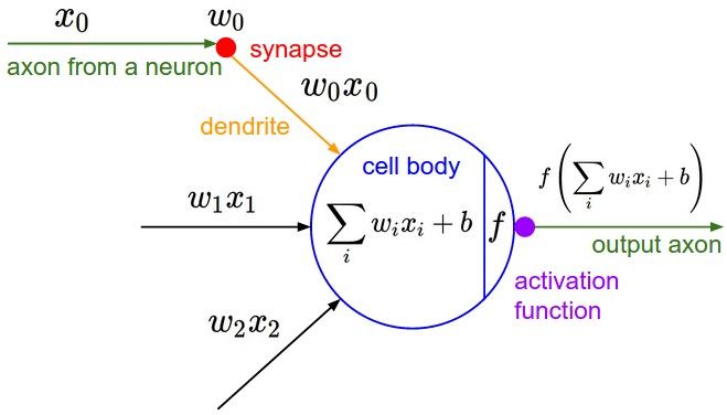


